Difference between revisions of "Regularized moduli spaces"

Revision as of 13:10, 3 June 2017

Abstract, Coherent Regularization

In order to regularize the moduli spaces of pseudoholomorphic polygons $\overline {\mathcal {M}}(x_{0};x_{1},\ldots ,x_{d})$ for each tuple of Lagrangians $\underline {L}={\bigl (}L_{0},\ldots ,L_{d}\subset M{\bigr )}$ , generators $\underline {x}={\bigl (}x_{0}\in {\text{Crit}}(L_{0},L_{d}),x_{1}\in {\text{Crit}}(L_{0},L_{1}),\ldots ,x_{d}\in {\text{Crit}}(L_{{d-1}},L_{d}){\bigr )}$ , and a fixed compatible almost complex structure $J$ , 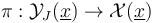any abstract regularization approach (opposed to geometric ones, as contrasted in [section 3, FFGW] and [sections 2.1-2, MW]) starts by describing each Gromov-compactified moduli space as

${\text{zero set}}\quad \overline {\mathcal {M}}(\underline {x})=\overline \partial _{{J,Y}}^{{-1}}(0)\quad {\text{of a section}}\quad \overline \partial _{{J,Y}}:{\mathcal {X}}(\underline {x})\to {\mathcal {Y}}_{J}(\underline {x})\quad {\text{of a bundle}}\quad \pi :{\mathcal {Y}}_{J}(\underline {x})\to {\mathcal {X}}(\underline {x}).$

In order to obtain boundary stratifications which imply the $A_{\infty }$ -relations, any abstract approach needs to regularize "coherently’’ (whereas geometric regularizations are automatically coherent), that is compatible with the boundary stratification of the ambient spaces ${\mathcal {X}}(\underline {x})$ being given by fiber products of other ambient spaces. In our setup, these fiber products are over finite sets of Morse and Floer critical points, so simplify to unions of Cartesian products,

$\partial {\mathcal {X}}(x_{0};x_{1},\ldots ,x_{d})=\bigsqcup _{{m,n\geq 0}}\bigsqcup _{{y\in {\text{Crit}}(L_{n},L_{{m+n}})}}{\mathcal {X}}(y;x_{{n+1}}\ldots x_{{n+m}})\times {\mathcal {X}}(x_{0};x_{1}\ldots x_{n},y,x_{{n+m+1}}\ldots x_{d}).$

In the abstract regularization approach of [2015-FOOO1], [2017-FOOO2], and most other virtual approaches, the global sections $s:{\mathcal {X}}\to {\mathcal {Y}}$ are patched together from smooth sections of finite rank bundles over finite dimensional manifolds $s_{i}:X_{i}\to Y_{i}$ . While at first glance this resolves most analytic issues (up to the question of obtaining smooth sections near nodal curves from the classical gluing analysis), it introduces a number of subtle combinatorial, algebraic, and topological challenges as discussed in [MW].

Many of these challenges stem from the lack of a natural ambient space, which is replaced by a highly choice-dependent space ${\mathcal {X}}$ that is constructed from nontrivial notions of transition data between the local base manifolds $X_{i}$ of different dimensions. Other undesirable features of this approach are that the sections $s_{i}$ are no longer directly identified with Cauchy-Riemann operators, and that the Kuranishi charts $s_{i}:X_{i}\to Y_{i}$ are generally 'too small' to allow for straight-forward constructions of new moduli spaces (e.g. by restriction to curves having certain intersection properties, or coupling of curves with each other or Morse trajectories) via restrictions or fiber products of the local sections. (Such constructions require transversality of evaluation maps whose domain is the ambient space ${\mathcal {X}}$ , which would need to be constructed with the particular transversality in mind.)

In the abstract regularization approach via polyfold theory [HWZ], the ambient space ${\mathcal {X}}$ is chosen ‘large enough’ to be fairly natural, allow for restrictions and fiber products, and so that the section $\overline \partial _{{J,Y}}$ is directly given by a Cauchy-Riemann operator. While this resolves most combinatorial, algebraic, and topological challenges - by building a natural ambient space that is e.g. Hausdorff and provides natural compactness controls - equipping this ambient space with a notion of smooth structure posed analytic issues that were insurmountable with classical infinite dimensional analysis.

Polyfold Fredholm Descriptions of Moduli spaces

To overcome the analytic challenges, the abstract parts of polyfold theory provide alternative notions of infinite dimensional spaces and differentiability with which we will be able to

equip each ambient space ${\mathcal {X}}(\underline {x})$ with a smooth structure as 'polyfold modeled on sc-Hilbert spaces';

equip each ambient bundle $\pi :{\mathcal {Y}}_{J}(\underline {x})\to {\mathcal {X}}(\underline {x})$ with a smooth bundle structure as 'strong polyfold bundle over ${\mathcal {X}}(\underline {x})$ ';

show that each Cauchy-Riemann section $\overline \partial _{{J,Y}}:{\mathcal {X}}(\underline {x})\to {\mathcal {Y}}_{J}(\underline {x})$ satisfies adapted notions of smoothness and nonlinear Fredholm properties, i.e. is a 'sc-Fredholm section of the polyfold bundle $\pi :{\mathcal {Y}}_{J}(\underline {x})\to {\mathcal {X}}(\underline {x})$ '.

Before we can use the abstract perturbation results from polyfold theory to regularize the zero sets $\overline \partial _{{J,Y}}^{{-1}}(0)\subset {\mathcal {X}}(\underline {x})$ , we need to restrict ourselves to (unions of) connected components of the ambient space within which the zero set is compact. Moreover, we will ultimately just need the zero sets of specific Fredholm indices. So for any $k\in \mathbb{Z } ,w_{0}\in \mathbb{R}$ we define

$\overline {\mathcal {M}}^{k}(\underline {x}):={\bigl \{}b\in \overline {\mathcal {M}}(\underline {x})\,{\big |}\,{\text{ind}}\,{{\rm {D}}}_{b}\overline \partial _{{J,Y}}=k{\bigr \}},\qquad \overline {\mathcal {M}}_{{w_{0}}}(\underline {x}):={\bigl \{}b\in \overline {\mathcal {M}}(\underline {x})\,{\big |}\,\omega (b)\leq w_{0}{\bigr \}}.$

Here the linearized section ${{\rm {D}}}_{b}\overline \partial _{{J,Y}}$ has a well defined Fredholm index in $\mathbb{Z }$ at any solution $b\in \overline \partial _{{J,Y}}^{{-1}}(0)$ , and $\omega$ is the symplectic area function defined on Moduli spaces of pseudoholomorphic polygons. 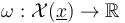We will extend both to locally constant functions on the ambient spaces, ${{\rm {ind}}}:{\mathcal {X}}(\underline {x})\to \mathbb{Z }$ and $\omega :{\mathcal {X}}(\underline {x})\to \mathbb{R}$ , and thus obtain ambient spaces for $\overline {\mathcal {M}}^{k}(\underline {x})$ and $\overline {\mathcal {M}}_{{w_{0}}}(\underline {x})$ ,

${\mathcal {X}}^{k}(\underline {x}):={\bigl \{}b\in {\mathcal {X}}(\underline {x})\,{\big |}\,{\text{ind}}(b)=k{\bigr \}},\qquad {\mathcal {X}}_{{w_{0}}}(\underline {x}):={\bigl \{}b\in {\mathcal {X}}(\underline {x})\,{\big |}\,\omega (b)\leq w_{0}{\bigr \}}.$

Now Gromov compactness can be formulated as saying that for any $w_{0}\in \mathbb{R}$ the restricted section $\overline \partial _{{J,Y}}|_{{{\mathcal {X}}_{{w_{0}}}(\underline {x})}}:{\mathcal {X}}_{{w_{0}}}(\underline {x})\to {\mathcal {Y}}_{J}(\underline {x})|_{{{\mathcal {X}}_{{w_{0}}}(\underline {x})}}:=\pi ^{{-1}}{\bigl (}{\mathcal {X}}_{{w_{0}}}(\underline {x}){\bigr )}$ is a proper Fredholm section (of a strong polyfold bundle over a polyfold that is modeled on sc-Hilbert spaces).

Indeed, [Definition 4.1 HWZIII] of a section being proper requires the zero set $\overline \partial _{{J,Y}}^{{-1}}(0)\cap {\mathcal {X}}_{{w_{0}}}(\underline {x})$ to be compact, and we will show that Gromov compactness implies properness.

Polyfold Regularizations

In the special case of trivial isotropy - when each ${\mathcal {X}}_{{w_{0}}}(\underline {x})$ is an M-polyfold - the abstract M-polyfold perturbation and implicit function theorem package [Theorem 5.18 HWZ] then provides, for any $w_{0}\in \mathbb{R}$ , a perturbation $s_{{w_{0}}}:{\mathcal {X}}_{{w_{0}}}(\underline {x})\to {\mathcal {Y}}_{J}(\underline {x})|_{{{\mathcal {X}}_{{w_{0}}}(\underline {x})}}$ that is transverse to $\overline \partial _{{J,Y}}$ and controls compactness such that the perturbed solution set ${\bigl \{}b\in {\mathcal {X}}_{{w_{0}}}(\underline {x})\,{\big |}\,\overline \partial _{{J,Y}}(b)=s_{{w_{0}}}(b){\bigr \}}$ inherits the structure of a compact manifold with boundary and corners induced by intersections with the boundary and corner structures of ${\mathcal {X}}_{{w_{0}}}(\underline {x})$ . We will see below that this perturbation section $s_{{w_{0}}}$ can in fact be extended to all of ${\mathcal {X}}(\underline {x})$ . However, in the case of nontrivial isotropy, we will have to work with multi-sections $\tau :{\mathcal {Y}}_{J}(\underline {x})\to \mathbb{Q} ^{+}$ . These are related to sections in the case of trivial isotropy by a section $s:{\mathcal {X}}(\underline {x})\to {\mathcal {Y}}_{J}(\underline {x})$ inducing a multi-section given by $\tau (\eta )=1$ iff $\eta =s(\pi (b))$ , and $\tau _{{w_{0}}}(\eta )=0$ otherwise.

In the general case of nontrivial isotropy, we moreover require orientations of Cauchy-Riemann sections before we can construct a multi-valued perturbation $\nu :{\mathcal {Y}}_{J}(\underline {x})\to \mathbb{Q} ^{+}$ such that the perturbed solution set

$\overline {\mathcal {M}}(\underline {x};\nu ):={\bigl \{}b\in {\mathcal {X}}(\underline {x})\,{\big |}\,\nu {\bigl (}\overline \partial _{{J,Y}}(b){\bigr )}>0{\bigr \}}$

is a branched suborbifold of the polyfold ${\mathcal {X}}_{{w_{0}}}(\underline {x})$ such that $\overline {\mathcal {M}}(\underline {x};\nu )\cap {\mathcal {X}}_{{w_{0}}}(\underline {x})$ is compact for any $w_{0}\in \mathbb{R}$ . (Moreover, this branched orbifold is weighted by the restriction $\nu |_{{\overline {\mathcal {M}}(\underline {x};\nu )}}:\overline {\mathcal {M}}(\underline {x};\nu )\to \mathbb{Q}$ .)

To construct $\nu$ we first apply [Theorem 4.19 HWZIII] to obtain - for any fixed $w_{0}\in \mathbb{R}$ - a multi-valued perturbation $\tau _{{w_{0}}}:{\mathcal {Y}}_{J}(\underline {x})|_{{{\mathcal {X}}_{{w_{0}}}(\underline {x})}}\to \mathbb{Q} ^{+}$ that is transverse to $\overline \partial _{{J,Y}}$ and controls compactness such that the solution set ${\bigl \{}b\in {\mathcal {X}}_{{w_{0}}}(\underline {x})\,{\big |}\,\tau _{{w_{0}}}{\bigl (}\overline \partial _{{J,Y}}(b){\bigr )}>0{\bigr \}}$ is a compact branched suborbifold of the polyfold ${\mathcal {X}}_{{w_{0}}}(\underline {x})$ with boundary and corners. We can moreover perform this construction for a sequence $w_{{0}}(i)\to \infty$ and in each step choose the multi-valued perturbation $\tau _{{w_{{0}}(i+1)}}$ to coincide on ${\mathcal {X}}_{{w_{0}(i)}}(\underline {x})$ with the (already transverse on these components) perturbation $\tau _{{w_{{0}}(i)}}$ . Then the required perturbation $\nu :{\mathcal {Y}}_{J}(\underline {x})\to \mathbb{Q} ^{+}$ can be obtained as the limit $\nu (\eta )=\lim _{{i\to \infty }}\tau _{{w_{{0}}(i)}}(\eta )=\tau _{{w_{{0}}(i_{\eta })}}(\eta )$ , where $i_{\eta }\gg 1$ such that $w_{{0}}(i_{\eta })\geq \omega (\pi (\eta ))$ .

Construction of Composition Operations

For the Composition Operators in the Polyfold Constructions for Fukaya Categories to be well defined we need to check that $\textstyle \sum _{{b\in \overline {\mathcal {M}}^{0}(\underline {x})}}\nu (b)\,T^{{\omega (b)}}$ defines an element in the Novikov ring. This requires the following two properties of the perturbed solution sets:

Every perturbed solution $b\in \overline {\mathcal {M}}^{0}(x_{0};x_{1},\ldots ,x_{d};\nu )$ needs to have nonnegative symplectic area $\omega (b)\geq 0$ . This is achieved as follows:

If all Lagrangians involved are pairwise either identical or transverse, then no Hamiltonian perturbations to the Cauchy-Riemann equation are involved in the construction of the unperturbed moduli space $\overline {\mathcal {M}}(x_{0};x_{1},\ldots ,x_{d})$ . Thus each component $u_{v}:\Sigma \to M$ of an unperturbed solution satisfies $\textstyle \int _{\Sigma }u_{v}^{*}\omega =\int _{\Sigma }{\tfrac 12}|{{\rm {d}}}u_{v}|^{2}\geq 0$ , and this sums up to $\omega (b)\geq 0$ . Thus the Cauchy-Riemann operator $\overline \partial _{J}$ has no zeros in the connected components ${\mathcal {X}}_{{<0}}(\underline {x})=\{b\in {\mathcal {X}}(\underline {x})\,|\,\omega (b)<0\}$ of negative symplectic area. Since transversality is a condition only at solutions, this means we can fix the perturbation $\nu |_{{{\mathcal {X}}_{{<0}}(\underline {x})}}\equiv 0$ an the connected components of the ambient space of negative energy. As a result, all perturbed solutions will satisfy $\omega (b)\geq 0$ , as required.

Here input from the Mirror Symmetry community is needed

on how to define $\omega$ , or which kind of Novikov coefficients to use, in the presence of Hamiltonian perturbations for nontransverse pairs of nonidentical Lagrangians.

Any subset of perturbed solutions

$\overline {\mathcal {M}}^{0}(\underline {x};\nu )\cap {\mathcal {X}}_{{w_{0}}}(\underline {x})$ of Fredholm index ${{\rm {ind}}}\,D_{b}\overline \partial _{{J,Y}}=0$ and bounded energy $\omega (b)\leq w_{0}$ for some $w_{0}>0$ needs to be a finite set. This is true by the following:

First, the implicit function theorem for transverse sc-Fredholm multi-sections of polyfold bundles implies that the set of perturbed solutions of Fredholm index 0, $\overline {\mathcal {M}}^{0}(\underline {x};\nu )$ carries the structure of a 0-dimensional weighted-branched orbifold

WORK IN PROGRESS

CAUTION: need to divide by order of isotropy to get weight functions ?!?

Proof of $A_{\infty }$ -relations

we need to explain how to obtain regularizations $\overline {\mathcal {M}}^{k}(x_{0};x_{1},\ldots ,x_{d};\nu )$ for expected dimensions $k=0,1$ by a choice of perturbations $\nu$ . Moreover, we need to choose these perturbations coherently to ensure that the boundary of each 1-dimensional part is given by Cartesian products of 0-dimensional parts,

$\partial \overline {\mathcal {M}}^{1}(x_{0};x_{1},\ldots ,x_{d};\nu )=\bigsqcup _{{m,n\geq 0}}\bigsqcup _{{y\in {\text{Crit}}(L_{n},L_{{m+n}})}}\overline {\mathcal {M}}^{0}(y;\underline {x}';\nu )\times \overline {\mathcal {M}}^{0}(x_{0};\underline {x},y,\underline {x}'';\nu ).$

Finally, we need to check that for each pair $(b,b')\in \overline {\mathcal {M}}^{0}(x_{0};\underline {x},y,\underline {x}'';\nu )\times \overline {\mathcal {M}}^{0}(y;\underline {x}';\nu )$ , when considered as boundary point $(b,b')\in \partial \overline {\mathcal {M}}^{1}(x_{0};x_{1},\ldots ,x_{d};\nu )$ , has symplectic area $\omega ((b,b'))=\omega (b)+\omega (b')$ and weight function ${\text{w}}((b,b'))=(-1)^{{\|\underline x\|}}{\text{w}}(b){\text{w}}(b')$ .

Analysis TODO:

when degenerating polygons to create a strip with  $L_{i}=L_{j}$  boundary conditions, will need to transfer from Morse-Bott breaking to boundary node

@@ Line 13: / Line 13: @@
 </math>
 </center>
-In order to obtain boundary stratifications which imply the <math>A_\infty</math>-relations, any abstract approach needs to regularize ``coherently’’ (whereas geometric regularizations are automatically coherent), that is compatible with the boundary stratification of the ambient spaces <math>\mathcal{X}(\underline{x})</math> being given by fiber products of other ambient spaces. In our setup, these fiber products are over finite sets of Morse and Floer critical points, so simplify to unions of Cartesian products,
+In order to obtain boundary stratifications which imply the <math>A_\infty</math>-relations, any abstract approach needs to regularize "coherently’’ (whereas geometric regularizations are automatically coherent), that is compatible with the boundary stratification of the ambient spaces <math>\mathcal{X}(\underline{x})</math> being given by fiber products of other ambient spaces. In our setup, these fiber products are over finite sets of Morse and Floer critical points, so simplify to unions of Cartesian products,
 <center>
 <math>

Difference between revisions of "Regularized moduli spaces"

Revision as of 13:10, 3 June 2017

Contents

Abstract, Coherent Regularization

Polyfold Fredholm Descriptions of Moduli spaces

Polyfold Regularizations

Construction of Composition Operations

Proof of $A_{\infty }$ -relations

Navigation menu

Personal tools

Namespaces

Variants

Views

More

Search

Navigation

Tools

Difference between revisions of "Regularized moduli spaces"

Revision as of 13:10, 3 June 2017

Contents

Abstract, Coherent Regularization

Polyfold Fredholm Descriptions of Moduli spaces

Polyfold Regularizations

Construction of Composition Operations

Proof of -relations

Navigation menu

Search

Proof of $A_{\infty }$ -relations