Regularized moduli spaces

table of contents

Abstract, Coherent Regularization

In order to regularize the moduli spaces of pseudoholomorphic polygons $\overline {\mathcal {M}}(x_{0};x_{1},\ldots ,x_{d})$ for each tuple of Lagrangians $L_{0},\ldots ,L_{d}\subset M$, generators $\underline {x}={\bigl (}x_{0}\in {\text{Crit}}(L_{0},L_{d}),x_{1}\in {\text{Crit}}(L_{0},L_{1}),\ldots ,x_{d}\in {\text{Crit}}(L_{{d-1}},L_{d}){\bigr )}$, and a fixed compatible almost complex structure $J$, any abstract regularization approach (opposed to geometric ones, as contrasted in [section 3, FFGW] and [sections 2.1-2, MW]) starts by describing each Gromov-compactified moduli space as

${\text{zero set}}\quad \overline {\mathcal {M}}(\underline {x})=\overline \partial _{{J,Y}}^{{-1}}(0)\quad {\text{of a section}}\quad \overline \partial _{{J,Y}}:{\mathcal {X}}(\underline {x})\to {\mathcal {Y}}_{J}(\underline {x})\quad {\text{of a bundle}}\quad \pi :{\mathcal {Y}}_{J}(\underline {x})\to {\mathcal {X}}(\underline {x}).$

In order to obtain boundary stratifications which imply the $A_{\infty }$-relations, any abstract approach needs to regularize "coherently" (whereas geometric regularizations are automatically coherent), that is compatible with the boundary stratification of the ambient spaces 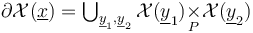$\partial {\mathcal {X}}(\underline {x})=\textstyle \bigcup _{{\underline {y}_{1},\underline {y}_{2}}}{\mathcal {X}}(\underline {y}_{1}){\underset {P}{\times }}{\mathcal {X}}(\underline {y}_{2})$ being given by fiber products (over some evaluation maps to a space $P$) of other ambient spaces. A little more precisely, in this general fiber product description, the regularizations $\overline {\mathcal {M}}(\underline {x};\nu (\underline {x}))$ need to have a notion of boundary for which Stokes' theorem holds and $\partial \overline {\mathcal {M}}(\underline {x};\nu )=\textstyle \bigcup _{{\underline {y}_{1},\underline {y}_{2}}}\overline {\mathcal {M}}(\underline {y}_{1};\nu ){\underset {P}{\times }}\overline {\mathcal {M}}(\underline {y}_{2};\nu )$.

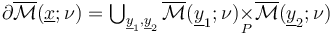In our setup, these fiber products are over finite sets of Morse and Floer critical points, so simplify to unions of Cartesian products,

$\partial {\mathcal {X}}(x_{0};x_{1},\ldots ,x_{d})=\bigcup _{{m,n\geq 0}}\bigcup _{{y\in {\text{Crit}}(L_{n},L_{{m+n}})}}{\mathcal {X}}(x_{0};x_{1}\ldots x_{n},y,x_{{n+m+1}}\ldots x_{d})\times {\mathcal {X}}(y;x_{{n+1}}\ldots x_{{n+m}}).$

These Cartesian products have overlaps in the corners of ${\mathcal {X}}(\underline {x})$. We can further specify this stratification by considering the boundary strata $\partial ^{{(k)}}{\mathcal {X}}(\underline {x}):=\{b\in {\mathcal {X}}(\underline {x})\,|\,d(b)=k\}$ with specific (boundary) degeneracy index (see [Section 3.1 HWZ-III] and [Section 5.3, FFGW]) - in particular denoting the interior of the ambient polyfolds by 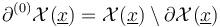$\partial ^{{(0)}}{\mathcal {X}}(\underline {x})={\mathcal {X}}(\underline {x})\setminus \partial {\mathcal {X}}(\underline {x})$ and the smooth part of the boundary (excluding corners) by $\partial ^{{(1)}}{\mathcal {X}}(\underline {x})=\partial {\mathcal {X}}(\underline {x})\setminus \{b\in {\mathcal {X}}(\underline {x})\,|\,d(b)\geq 2\}$. With this notation, we can express the fact that the smooth part of the boundary is the disjoint union of Cartesian products of interiors,

$\partial ^{{(1)}}{\mathcal {X}}(\underline {x})=\bigsqcup _{{\underline {x}=(x_{0};\underline {x}',\underline {x}'',\underline {x}''')}}\bigsqcup _{{y\in {\text{Crit}}(\ldots )}}\partial ^{{(0)}}{\mathcal {X}}(x_{0};\underline {x}',y,\underline {x}''')\times \partial ^{{(0)}}{\mathcal {X}}(y;\underline {x}'').$

If we now think of the regularizations as zero sets of a transversely perturbed section, 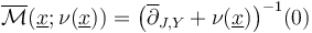$\overline {\mathcal {M}}(\underline {x};\nu (\underline {x}))={\bigl (}\overline \partial _{{J,Y}}+\nu (\underline {x}){\bigr )}^{{-1}}(0)$, then the coherence requirement can be guaranteed if the restriction of any perturbation $\nu (\underline {x}):{\mathcal {X}}(\underline {x})\to {\mathcal {Y}}_{J}(\underline {x})$ to each boundary component is given by the product of perturbations associated to the splitting of the boundary component,

$\nu (\underline {x})|_{{\partial ^{{(0)}}{\mathcal {X}}(x_{0};\underline {x}',y,\underline {x}''')\times \partial ^{{(0)}}{\mathcal {X}}(y;\underline {x}'')}}=\nu (x_{0};\underline {x}',y,\underline {x}''')\times \nu (y;\underline {x}'').$

In the abstract regularization approach of [2015-FOOO1], [2017-FOOO2], and most other virtual approaches, the global sections $s:{\mathcal {X}}\to {\mathcal {Y}}$ are patched together from smooth sections of finite rank bundles over finite dimensional manifolds $s_{i}:X_{i}\to Y_{i}$. These local sections are obtained by 'finite dimensional reduction' of local Fredholm descriptions of the moduli spaces, but are no longer directly identified with Cauchy-Riemann operators. Another undesirable feature of this approach is that the local Kuranishi ambient spaces $X_{i}$ are generally 'too small' to allow for straight-forward constructions of new moduli spaces (e.g. by restriction to curves having certain intersection properties, or coupling of curves with each other or Morse trajectories) via restrictions or fiber products of the local sections.

While at first glance the finite dimensional reductions in virtual approaches resolve most analytic issues (up to the question of obtaining smooth sections near nodal curves from the classical gluing analysis), it introduces a number of subtle combinatorial, algebraic, and topological challenges as discussed in [MW].

Many of these challenges stem from the lack of a natural ambient space, which is replaced by a highly choice-dependent space ${\mathcal {X}}=\bigcup X_{i}/\sim$ that is constructed from nontrivial notions of transition data between the local base manifolds $X_{i}$ of different dimensions. To see why the Kuranishi charts $s_{i}:X_{i}\to Y_{i}$ are generally 'too small' to allow for restrictions or fiber products of the local sections, note that such constructions require transversality of evaluation maps whose domains are the local ambient spaces $X_{i}$. So these would need to be constructed with the particular transversality in mind - which may not be possible if e.g. transversality to an uncountable set of chains is desired.

In the abstract regularization approach via polyfold theory [HWZ], the ambient space ${\mathcal {X}}$ is infinite dimensional and chosen ‘large enough’ to be fairly natural, allow for restrictions and fiber products, and so that the section $\overline \partial _{{J,Y}}$ is directly given by a Cauchy-Riemann operator. While this resolves most combinatorial, algebraic, and topological challenges - by building a natural ambient space that is e.g. Hausdorff and provides natural compactness controls - equipping this ambient space with a notion of smooth structure posed analytic issues that were insurmountable with classical infinite dimensional analysis.

Polyfold Fredholm Descriptions of Moduli spaces

To overcome the analytic challenges, the abstract parts of polyfold theory provide alternative notions of infinite dimensional spaces and differentiability with which we will be able to

• equip each ambient space ${\mathcal {X}}(\underline {x})$ with a smooth structure as 'polyfold modeled on sc-Hilbert spaces';

• equip each ambient bundle $\pi :{\mathcal {Y}}_{J}(\underline {x})\to {\mathcal {X}}(\underline {x})$ with a smooth bundle structure as 'strong polyfold bundle over ${\mathcal {X}}(\underline {x})$';

• show that each Cauchy-Riemann section $\overline \partial _{{J,Y}}:{\mathcal {X}}(\underline {x})\to {\mathcal {Y}}_{J}(\underline {x})$ satisfies adapted notions of smoothness and nonlinear Fredholm properties, i.e. is a 'sc-Fredholm section of the polyfold bundle $\pi :{\mathcal {Y}}_{J}(\underline {x})\to {\mathcal {X}}(\underline {x})$'.

Before we can use the abstract perturbation results from polyfold theory to regularize the zero sets $\overline \partial _{{J,Y}}^{{-1}}(0)\subset {\mathcal {X}}(\underline {x})$, we need to restrict ourselves to (unions of) connected components of the ambient space within which the zero set is compact. Moreover, we will ultimately just need the zero sets of specific Fredholm indices. So for any $k\in \mathbb{Z } ,w_{0}\in \mathbb{R}$ we define

$\overline {\mathcal {M}}^{k}(\underline {x}):={\bigl \{}b\in \overline {\mathcal {M}}(\underline {x})\,{\big |}\,{\text{ind}}\,{{\rm {D}}}_{b}\overline \partial _{{J,Y}}=k{\bigr \}},\qquad \overline {\mathcal {M}}_{{w_{0}}}(\underline {x}):={\bigl \{}b\in \overline {\mathcal {M}}(\underline {x})\,{\big |}\,\omega (b)\leq w_{0}{\bigr \}},\qquad \overline {\mathcal {M}}_{{w_{0}}}^{k}(\underline {x}):=\overline {\mathcal {M}}^{k}(\underline {x})\cap \overline {\mathcal {M}}_{{w_{0}}}(\underline {x}).$

Here the linearized section ${{\rm {D}}}_{b}\overline \partial _{{J,Y}}$ has a well defined Fredholm index in $\mathbb{Z }$ at any solution $b\in \overline \partial _{{J,Y}}^{{-1}}(0)$, and $\omega$ is the symplectic area function defined on moduli spaces of pseudoholomorphic polygons. We will extend both to locally constant functions on the ambient spaces, ${{\rm {ind}}}:{\mathcal {X}}(\underline {x})\to \mathbb{Z }$ and $\omega :{\mathcal {X}}(\underline {x})\to \mathbb{R}$, and thus obtain ambient spaces for $\overline {\mathcal {M}}^{k}(\underline {x})$ and $\overline {\mathcal {M}}_{{w_{0}}}(\underline {x})$,

${\mathcal {X}}^{k}(\underline {x}):={\bigl \{}b\in {\mathcal {X}}(\underline {x})\,{\big |}\,{\text{ind}}(b)=k{\bigr \}},\qquad {\mathcal {X}}_{{w_{0}}}(\underline {x}):={\bigl \{}b\in {\mathcal {X}}(\underline {x})\,{\big |}\,\omega (b)\leq w_{0}{\bigr \}}.$

Now Gromov compactness can be formulated as saying that for any $w_{0}\in \mathbb{R}$ the restricted section $\overline \partial _{{J,Y}}|_{{{\mathcal {X}}_{{w_{0}}}(\underline {x})}}:{\mathcal {X}}_{{w_{0}}}(\underline {x})\to {\mathcal {Y}}_{J}(\underline {x})|_{{{\mathcal {X}}_{{w_{0}}}(\underline {x})}}:=\pi ^{{-1}}{\bigl (}{\mathcal {X}}_{{w_{0}}}(\underline {x}){\bigr )}$ is a proper Fredholm section (of a strong polyfold bundle over a polyfold that is modeled on sc-Hilbert spaces).

Indeed, [Definition 4.1 HWZ-III] of a section being proper requires the zero set $\overline \partial _{{J,Y}}^{{-1}}(0)\cap {\mathcal {X}}_{{w_{0}}}(\underline {x})$ to be compact, and we will show that Gromov compactness implies properness.

Polyfold Regularizations

In the special case of trivial isotropy - when each ${\mathcal {X}}_{{w_{0}}}(\underline {x})$ is an M-polyfold - the abstract M-polyfold perturbation and implicit function theorem package [Theorem 5.18 HWZ-1] then provides, for any $w_{0}\in \mathbb{R}$, a perturbation $s_{{w_{0}}}:{\mathcal {X}}_{{w_{0}}}(\underline {x})\to {\mathcal {Y}}_{J}(\underline {x})|_{{{\mathcal {X}}_{{w_{0}}}(\underline {x})}}$ that is transverse to $\overline \partial _{{J,Y}}$, in general position to the boundary&corners of ${\mathcal {X}}_{{w_{0}}}(\underline {x})$, and controls compactness such that the perturbed solution set

$\overline {\mathcal {M}}_{{w_{0}}}(\underline {x};s_{{w_{0}}}):={\bigl \{}b\in {\mathcal {X}}_{{w_{0}}}(\underline {x})\,{\big |}\,\overline \partial _{{J,Y}}(b)=s_{{w_{0}}}(b){\bigr \}}$

inherits the structure of a compact manifold whose dimension near $b\in \overline {\mathcal {M}}_{{w_{0}}}(\underline {x};s_{{w_{0}}})$ is given by the Fredholm index ${\text{ind}}\,{{\rm {D}}}_{b}\overline \partial _{{J,Y}}$.

Moreover, the boundary and corner strata of the perturbed solution set are given by transverse general position intersections with the boundary and corner strata of the ambient M-polyfold ${\mathcal {X}}_{{w_{0}}}(\underline {x})$ in the sense that

for each corner degeneracy index $m\geq 0$ (with $m=0$ denoting the interior and $m=1$ the main stratum of the boundary) we have $\partial ^{{(m)}}\overline {\mathcal {M}}_{{w_{0}}}(\underline {x};s_{{w_{0}}})=\overline {\mathcal {M}}_{{w_{0}}}(\underline {x};s_{{w_{0}}})\cap \partial ^{{(m)}}{\mathcal {X}}_{{w_{0}}}(\underline {x})$ cut out transversely by the restriction ${\bigl (}\overline \partial _{{J,Y}}-s_{{w_{0}}}{\bigr )}{\big |}_{{\partial ^{{(m)}}{\mathcal {X}}_{{w_{0}}}(\underline {x})}}$, which has Fredholm index ${\text{ind}}\,{{\rm {D}}}_{b}\overline \partial _{{J,Y}}-m$. In particular:

• The index $k=0$ part of the perturbed moduli space $\overline {\mathcal {M}}_{{w_{0}}}^{0}(\underline {x};s_{{w_{0}}}):=\overline {\mathcal {M}}_{{w_{0}}}(\underline {x};s_{{w_{0}}})\cap {\mathcal {X}}^{0}(\underline {x})$ is a compact 0-manifold that does not intersect the boundary of the ambient M-polyfold.
• The $k=1$-dimensional part of the perturbed moduli space $\overline {\mathcal {M}}_{{w_{0}}}^{1}(\underline {x};s_{{w_{0}}}):=\overline {\mathcal {M}}_{{w_{0}}}(\underline {x};s_{{w_{0}}})\cap {\mathcal {X}}^{1}(\underline {x})$ is a compact 1-manifold with boundary $\partial \overline {\mathcal {M}}_{{w_{0}}}^{1}(\underline {x};s_{{w_{0}}})=\overline {\mathcal {M}}_{{w_{0}}}^{1}(\underline {x};s_{{w_{0}}})\cap \partial ^{{(1)}}{\mathcal {X}}_{{w_{0}}}(\underline {x})$.

This will be used - in the setting of possibly nontrivial isotropy - in the proof of the $A_{\infty }$-relations.

We will see below that this perturbation section $s_{{w_{0}}}$ can in fact be extended to all of ${\mathcal {X}}(\underline {x})$. However, in the case of nontrivial isotropy, we will have to work with multisections $\nu :{\mathcal {Y}}_{J}(\underline {x})\to \mathbb{Q} ^{+}:=\mathbb{Q} \cap [0,\infty )$. These are related to sections in the case of trivial isotropy by a section $s:{\mathcal {X}}(\underline {x})\to {\mathcal {Y}}_{J}(\underline {x})$ inducing a multisection given by $\nu (\eta )=1$ iff $\eta =s(\pi (b))$, and $\nu _{{w_{0}}}(\eta )=0$ otherwise. In the general case of nontrivial isotropy, we moreover require orientations of Cauchy-Riemann sections before we can construct a multisection $\nu :{\mathcal {Y}}_{J}(\underline {x})\to \mathbb{Q} ^{+}$ such that the perturbed solution set

$\overline {\mathcal {M}}(\underline {x};\nu ):={\text{supp}}(\nu \circ \overline \partial _{{J,Y}})\cap {\mathcal {X}}(\underline {x}):={\bigl \{}b\in {\mathcal {X}}(\underline {x})\,{\big |}\,\nu {\bigl (}\overline \partial _{{J,Y}}(b){\bigr )}>0{\bigr \}}(\underline {x})$

inherits the structure of a branched suborbifold of the polyfold ${\mathcal {X}}_{{w_{0}}}(\underline {x})$ such that $\overline {\mathcal {M}}(\underline {x};\nu )\cap {\mathcal {X}}_{{w_{0}}}(\underline {x})$ is compact for any $w_{0}\in \mathbb{R}$.

This branched orbifold will also inherit a weight function, which (by abuse of notation) we denote $\nu :\overline {\mathcal {M}}(\underline {x};\nu )\to \mathbb{Q} ^{+}$.

At points with nontrivial isotropy, the weight is in fact given by the restriction of $\nu \circ \overline \partial _{{J,Y}}$, multiplied by a sign arising from the coherent orientations on the regularized moduli spaces. At points with nontrivial isotopy, this signed value of $\nu \circ \overline \partial _{{J,Y}}$ needs to be divided by the order of the isotropy group.

The construction of $\nu$ is based on [Theorem 4.19 HWZ-III],

which we apply to obtain - for any fixed $w_{0}\in \mathbb{R}$ - a multisection $\nu _{{w_{0}}}:{\mathcal {Y}}_{J}(\underline {x})|_{{{\mathcal {X}}_{{w_{0}}}(\underline {x})}}\to \mathbb{Q} ^{+}$ that is transverse to $\overline \partial _{{J,Y}}$ and controls compactness such that the solution set ${\bigl \{}b\in {\mathcal {X}}_{{w_{0}}}(\underline {x})\,{\big |}\,\nu _{{w_{0}}}{\bigl (}\overline \partial _{{J,Y}}(b){\bigr )}>0{\bigr \}}$ is a compact branched suborbifold of the polyfold ${\mathcal {X}}_{{w_{0}}}(\underline {x})$ with boundary and corners. We can moreover perform this construction for a sequence $w_{{0}}(i)\to \infty$ and in each step choose the multisection $\nu _{{w_{{0}}(i+1)}}$ to coincide on ${\mathcal {X}}_{{w_{0}(i)}}(\underline {x})$ with the (already transverse on these components) perturbation $\nu _{{w_{{0}}(i)}}$. Then the required perturbation $\nu :{\mathcal {Y}}_{J}(\underline {x})\to \mathbb{Q} ^{+}$ can be obtained as the limit $\nu (\eta )=\lim _{{i\to \infty }}\nu _{{w_{{0}}(i)}}(\eta )=\nu _{{w_{{0}}(i_{\eta })}}(\eta )$, where $i_{\eta }\gg 1$ such that $w_{{0}}(i_{\eta })\geq \omega (\pi (\eta ))$.

Moreover, by choosing $\nu$ in 'general position', we can ensure that the boundary and corner strata of the perturbed solution set are given by transverse intersections with the boundary and corner strata of the ambient polyfold ${\mathcal {X}}(\underline {x})$. In particular, the proof of the $A_{\infty }$-relations in the polyfold constructions for Fukaya categories is based on the following two special cases:

• The index $k=0$ part of the perturbed moduli space $\overline {\mathcal {M}}^{0}(\underline {x};\nu ):={\text{supp}}(\nu \circ \overline \partial _{{J,Y}})\cap {\mathcal {X}}^{0}(\underline {x})\subset \partial ^{{(0)}}{\mathcal {X}}^{0}(\underline {x})$ is a 0-dimensional manifold contained in the interior of the ambient polyfold with weight function $\nu :\overline {\mathcal {M}}^{0}(\underline {x};\nu )\to \mathbb{Q} ^{+}$.
• The $k=1$-dimensional part of the perturbed moduli space $\overline {\mathcal {M}}^{1}(\underline {x};\nu ):={\text{supp}}(\nu \circ \overline \partial _{{J,Y}})\cap {\mathcal {X}}^{1}(\underline {x})$ is a 1-dimensional branched suborbifold of the ambient polyfold with weight function $\nu :\overline {\mathcal {M}}^{1}(\underline {x};\nu )\to \mathbb{Q} ^{+}$ and boundary $\partial \overline {\mathcal {M}}^{1}(\underline {x};\nu )=\overline {\mathcal {M}}^{1}(\underline {x};\nu )\cap \partial ^{{(1)}}{\mathcal {X}}(\underline {x})$.

Since the boundary&corner stratification of the ambient polyfold ${\mathcal {X}}(\underline {x})$ is given, the coherence required for the $A_{\infty }$-relations can then be achieved by constructing the perturbation $\nu$ coherently, i.e. such that for every decomposition $\underline {x}=(x_{0};\underline {x}',\underline {x}'',\underline {x}''')$ into $\underline {x}'=(x_{1}\ldots x_{n}),\underline {x}''=(x_{{n+1}}\ldots x_{{n+m}}),\underline {x}'''=(x_{{n+m+1}}\ldots x_{d})$ and corresponding generator $y\in {\text{Crit}}(L_{n},L_{{m+n}})$, the perturbation $\nu (\underline {x}):=\nu |_{{{\mathcal {X}}(\underline {x})}}$ is given on each smooth boundary stratum by products of the perturbations on the ambient polyfolds indicated by the splitting of the generators,

$\nu (\underline {x})|_{{\partial ^{{(0)}}{\mathcal {X}}(x_{0};\underline {x}',y,\underline {x}''')\times \partial ^{{(0)}}{\mathcal {X}}(y;\underline {x}'')}}=\nu (x_{0};\underline {x}',y,\underline {x}''')\times \nu (y;\underline {x}'')\;:\,(b,b')\;\mapsto \;\nu (x_{0};\underline {x}',y,\underline {x}'''){\bigl (}b{\bigr )}\cdot \nu (y;\underline {x}''){\bigl (}b'{\bigr )}.$

To see why this implies the required coherence of regularizations $\partial \overline {\mathcal {M}}^{1}(\underline {x};\nu ){\overset {?}{=}}\bigsqcup _{{\underline {x}=(x_{0};\underline {x}',\underline {x}'',\underline {x}''')}}\bigsqcup _{{y\in {\text{Crit}}(\ldots )}}\overline {\mathcal {M}}^{0}(x_{0};\underline {x}',y,\underline {x}''';\nu )\times \overline {\mathcal {M}}^{0}(y;\underline {x}'';\nu )$, note that the above identities for the boundary strata of the perturbed solution spaces and ambient polyfolds allow us to express the coherence requirements as

${\text{supp}}(\nu \circ \overline \partial _{{J,Y}})\cap \bigsqcup _{{\underline {x}',\underline {x}'',\underline {x}''',y}}\partial ^{{(0)}}{\mathcal {X}}(x_{0};\underline {x}',y,\underline {x}''')\times \partial ^{{(0)}}{\mathcal {X}}(y;\underline {x}''){\overset {?}{=}}\bigsqcup _{{\underline {x}',\underline {x}'',\underline {x}''',y}}{\bigl (}{\text{supp}}(\nu \circ \overline \partial _{{J,Y}})\cap \partial ^{{(0)}}{\mathcal {X}}(x_{0};\underline {x}',y,\underline {x}'''){\bigr )}\times {\bigl (}{\text{supp}}(\nu \circ \overline \partial _{{J,Y}})\cap \partial ^{{(0)}}{\mathcal {X}}(y;\underline {x}''){\bigr )}.$

In the case of trivial isotropy, an inductive construction of such coherent perturbations is given in a preprint draft by Ben Filippenko. Unfortunately, the generalization of this construction to nontrivial isotropy requires the resolution of a surprisingly nontrivial issue of extending multisections given on boundaries and corners to the interior of a polyfold. In fact, this same issue already appears in finite dimensions for multisections of orbi-bundles with boundary and corners. It is being resolved in a not yet available manuscript by Hofer-Wysocki-Zehnder.

Construction of Composition Operations

For the Composition Operators in the polyfold constructions for Fukaya categories to be well defined we need to check that $\textstyle \sum _{{b\in \overline {\mathcal {M}}^{0}(\underline {x};\nu )}}\nu (b)\,T^{{\omega (b)}}$ defines an element in the Novikov ring. This requires the following two properties of the perturbed solution sets:

Every perturbed solution $b\in \overline {\mathcal {M}}^{0}(x_{0};x_{1},\ldots ,x_{d};\nu )$ needs to have nonnegative symplectic area $\omega (b)\geq 0$. This is achieved as follows:

If all Lagrangians involved are pairwise either identical or transverse, then no Hamiltonian perturbations to the Cauchy-Riemann equation are involved in the construction of the unperturbed moduli space $\overline {\mathcal {M}}(x_{0};x_{1},\ldots ,x_{d})$. Thus each component $u_{v}:\Sigma \to M$ of an unperturbed solution satisfies $\textstyle \int _{\Sigma }u_{v}^{*}\omega =\int _{\Sigma }{\tfrac 12}|{{\rm {d}}}u_{v}|^{2}\geq 0$, and this sums up to $\omega (b)\geq 0$. Thus the Cauchy-Riemann operator $\overline \partial _{J}$ has no zeros in the connected components ${\mathcal {X}}_{{<0}}(\underline {x})=\{b\in {\mathcal {X}}(\underline {x})\,|\,\omega (b)<0\}$ of negative symplectic area. Since transversality is a condition only at solutions, this means we can fix the perturbation $\nu |_{{{\mathcal {X}}_{{<0}}(\underline {x})}}\equiv 0$ on the connected components of the ambient space of negative energy. As a result, all perturbed solutions will satisfy $\omega (b)\geq 0$, as required.

Here input from the Mirror Symmetry community is needed

on how to define $\omega$, or which kind of Novikov coefficients to use, in the presence of Hamiltonian perturbations for nontransverse pairs of nonidentical Lagrangians.

Any subset of perturbed solutions $\overline {\mathcal {M}}^{0}(\underline {x};\nu )\cap {\mathcal {X}}_{{w_{0}}}(\underline {x})$ of Fredholm index ${{\rm {ind}}}\,{{\rm {D}}}_{b}\overline \partial _{{J,Y}}=0$ and bounded energy $\omega (b)\leq w_{0}$ for some $w_{0}>0$ needs to be a finite set.

This is true by the following:

First, preservation of compactness in the polyfold regularization (as discussed above) guarantees that $\overline {\mathcal {M}}^{0}(\underline {x};\nu )\cap {\mathcal {X}}_{{w_{0}}}(\underline {x})$ is a compact set. Second, the implicit function theorem for transverse sc-Fredholm multisections of polyfold bundles implies that the set of perturbed solutions of Fredholm index 0, $\overline {\mathcal {M}}^{0}(\underline {x};\nu )$ carries the structure of a 0-dimensional weighted-branched orbifold. Together, this implies that $\overline {\mathcal {M}}^{0}(\underline {x};\nu )\cap {\mathcal {X}}_{{w_{0}}}(\underline {x})$ is a finite set, as claimed. (The weighted-branching structure is expressed in the weight function $\nu$.) </math>

Proof of $A_{\infty }$-relations

As explained in polyfold constructions for Fukaya categories, this proof follows from coherence of the regularizations,

$\partial \overline {\mathcal {M}}^{1}(\underline {x};\nu )=\bigsqcup _{{\underline {x}=(x_{0};\underline {x}',\underline {x}'',\underline {x}''')}}\bigsqcup _{{y\in {\text{Crit}}(\ldots )}}\overline {\mathcal {M}}^{0}(x_{0};\underline {x}',y,\underline {x}''';\nu )\times \overline {\mathcal {M}}^{0}(y;\underline {x}'';\nu )$

together with the following two relations at boundary points $(b,b')\in \partial \overline {\mathcal {M}}^{1}(\underline {x};\nu )$ corresponding to pairs of $b\in \overline {\mathcal {M}}^{0}(x_{0};\underline {x}',y,\underline {x}''';\nu )$ and $b'\in \overline {\mathcal {M}}^{0}(y;\underline {x}'';\nu )$ :

1. Multiplicativity of weight functions $\nu ((b,b'))=(-1)^{{\|\underline {x}'\|}}\nu (b)\nu (b')$ is achieved by

• coherent construction of the multisections, $\nu (b,b')=\nu (b)\cdot \nu (b')$;
• the observation that the isotropy groups in Cartesian products are multiplicative;
• coherent orientations on the regularized moduli spaces which in particular yield the sign $(-1)^{{\|\underline {x}'\|}}$.

2. Additivity of symplectic area $\omega ((b,b'))=\omega (b)+\omega (b')$ holds by construction of the symplectic area function.