Difference between revisions of "Ambient space"
(Created page with " ---- <math></math> <center> <math> </math> </center> <div class="toccolours mw-collapsible mw-collapsed"> <div class="mw-collapsible-content"> </div></div>") |
m |
||
| Line 1: | Line 1: | ||
| + | [[table of contents]] | ||
| + | |||
| + | |||
| + | |||
| + | |||
| + | |||
| + | |||
| + | For the construction of a general <math>A_\infty</math>-composition map we are given <math>d+1\geq 1</math> Lagrangians <math>L_0,\ldots,L_d\subset M</math> and a fixed autonomous Hamiltonian function <math>H_{L_i,L_j}:M\to\R</math> for each pair <math>L_i\neq L_j</math> whose time-1 flow provides transverse intersections <math>\phi_{L_i,L_j}(L_i)\pitchfork L_j</math>. | ||
| + | To simplify notation for consecutive Lagrangians in the list, we index it cyclically by <math>i\in \Z_{d+1}</math> and abbreviate <math>\phi_i:=\phi_{L_{i-1},L_i}</math> so that we have <math>\phi_i(L_{i-1})\pitchfork L_i</math> whenever <math>L_{i-1}\neq L_i</math>, and in particular <math>\phi_0(L_d)\pitchfork L_0</math> unless <math>L_d=L_0</math>. | ||
| + | Now, given generators <math>x_0\in\text{Crit}(L_0,L_d),</math> <math>x_1\in\text{Crit}(L_0,L_1), \ldots,</math> <math>x_d\in\text{Crit}(L_{d-1},L_d)</math> of these morphism spaces, we construct the Gromov-compactified moduli space of generalized pseudoholomorphic polygons by combining the two special cases above with sphere bubble trees, | ||
| + | <center> | ||
| + | <math> | ||
| + | \mathcal{M}(x_0;x_1,\ldots,x_d) := \bigl\{ (T, \underline{\gamma}, \underline{z}, \underline{w}, \underline{\beta}, \underline{u} ) \,\big|\, \text{1. - 8.} \bigr\}/ \sim | ||
| + | </math> | ||
| + | </center> | ||
| + | where | ||
| + | |||
| + | 1. <math>T</math> is an ordered tree with sets of vertices <math>V=V^m \cup V^c</math> and edges <math>E</math>, | ||
| + | <div class="toccolours mw-collapsible mw-collapsed"> | ||
| + | equipped with orientations towards the root, orderings of incoming edges, and a partition into main and critical (leaf and root) vertices as follows: | ||
| + | <div class="mw-collapsible-content"> | ||
| + | * The edges <math>E\subset V\times V\setminus \Delta_V</math> are oriented towards the root vertex <math>v_0\in V</math> of the tree, so that each vertex <math>v\in V</math> has a unique outgoing edge <math>e^0_v=(v,\;\cdot\;)\in E</math> (except for the root vertex which has no outgoing edge) and a (possibly empty) set of incoming edges <math>E^{\rm in}_v = \{e=(\;\cdot\;, v) \in E\}</math>. | ||
| + | *The set of incoming edges is ordered, <math>E^{\rm in}_v=\{e^1_v, \ldots, e^{|v|-1}_v\}</math>. This induces a cyclic order on the set of all edges <math>E_v:=\{e^0_v, e^1_v, \ldots, e^{|v|-1}_v\}</math> adjacent to <math>v</math>, by setting <math>e^{|v|}_v=e^0_v</math>, and we will denote consecutive edges in this order by <math>e=e^i_v, e+1=e^{i+1}_v</math>. In particular this yields <math>e^0_v + i = e^i_v</math>. | ||
| + | * The set of vertices is partitioned <math>V=V^m \sqcup V^c</math> into the sets of ''main vertices'' <math>V^m</math> and ''critical vertices'' <math>V^c=\{v_0^c,v_1^c,\ldots v_d^c\}</math>. The latter is ordered to start with the root <math>v_0^c=v_0</math> and then contains d leaves <math>v_i^c</math> of the tree, with order induced by the orientation and order of the edges. | ||
| + | * The root vertex <math>v^c_0\in V^c</math> has a single edge <math>\{e^1_{v_0}=(v,v_0^c)\}=E^{\rm in}_{v_0}=E_{v_0}</math>, and this attaches to a main vertex <math>v\in V^m</math> except for one special case: For <math>d=1</math> and <math>L_d=L_0</math> we allow the tree with a single edge <math>e=(v_1^c,v_0^c)</math> between its two critical vertices <math>V=\{v_0^c,v_1^c\}</math>. | ||
| + | </div></div> | ||
| + | |||
| + | 2. The tree structure induces tuples of Lagrangians <math>\underline{L}=(\underline{L}^v)_{v\in V^m}</math> | ||
| + | <div class="toccolours mw-collapsible mw-collapsed"> | ||
| + | that label the boundary components of domains in overall counter-clockwise order <math>L_0,\ldots,L_d</math> as follows: | ||
| + | <div class="mw-collapsible-content"> | ||
| + | * For each main vertex <math>v\in V^m</math> the Lagrangian label <math>\underline{L}^v = (L^v_e)_{e\in E_v}</math> is a cyclic sequence of Lagrangians <math>L^v_e \in \{L_0,\ldots,L_d\}</math> indexed by the adjacent edges <math>E_v</math> (which will become the boundary condition on <math>(\partial \Sigma^v)_e</math>). | ||
| + | * For each edge <math>e=(v^-,v^+)\in E</math> the Lagrangian labels satisfy a matching condition as follows: | ||
| + | ** The edge from a critical leaf <math>v^-=v_i^c\in V^c</math> requires <math>L^{v^+}_e=L_i,L^{v^+}_{e-1}=L_{i-1}</math>. | ||
| + | ** The edge to the critical root <math>v^+=v_0^c\in V^c</math> requires <math>L^{v^-}_e=L_0,L^{v^-}_{e-1}=L_d</math>. | ||
| + | ** Any edge between main vertices <math>v^-,v^+\in V^m</math> requires <math>L^{v^-}_{e}=L^{v^+}_{e-1}</math> and <math>L^{v^-}_{e-1}=L^{v^+}_{e}</math>. | ||
| + | ** Since <math>T</math> has no further leaves, this determines the Lagrangian labels uniquely. | ||
| + | </div></div> | ||
| + | |||
| + | 3. <math>\underline{\gamma}=(\underline{\gamma}_e)_{e\in E}</math> is a tuple of generalized Morse trajectories | ||
| + | <div class="toccolours mw-collapsible mw-collapsed"> | ||
| + | in the following [[compactified Morse trajectory spaces]]: | ||
| + | <div class="mw-collapsible-content"> | ||
| + | * Any edge <math>e=(v^c_i,w)</math> from a critical leaf <math>v^c_i</math> to a main vertex <math>w\in V^m</math> is labeled by a half-infinite Morse trajectory <math>\underline{\gamma}_e \in \overline\mathcal{M}(x_i,L_i)</math> if <math>L_{i-1}=L_i</math>, resp. by the constant <math>\underline{\gamma}_e \equiv x_i \in {\rm Crit}(L_{i-1},L_i)</math> in the discrete space <math>\phi_i(L_{i-1})\cap L_i</math> if <math>L_{i-1}\neq L_i</math>. | ||
| + | * If the edge to the root <math>e=(v,v^c_0)</math> attaches to a main vertex <math>v\in V^m</math> then it is labeled by a half-infinite Morse trajectory <math>\underline{\gamma}_e \in \overline\mathcal{M}(L_0,x_0)</math> if <math>L_d=L_0</math>, resp. by the constant <math>\underline{\gamma}_e \equiv x_0 \in {\rm Crit}(L_d,L_0)</math> in the discrete space <math>\phi_0(L_d)\cap L_0</math> if <math>L_d\neq L_0</math>. | ||
| + | * An edge <math>e=(v^c_i,v^c_j)</math> between critical vertices is labeled by an infinite Morse trajectory <math>\underline{\gamma}_e \in \overline\mathcal{M}(x_i,x_j)</math> (this occurs only for <math>d=1</math> with <math>L_0=L_1</math> and the tree with one edge <math>e=(v^c_1,v^c_0)</math>). | ||
| + | * Any edge <math>e=(v,w)</math> between main vertices <math>v,w\in V^m</math> is labeled by a finite or infinite Morse trajectory <math>\underline{\gamma}_e \in \overline\mathcal{M}(L^v_e,L^v_e)</math> in case <math>L^v_e=L^v_{e-1}</math>, resp. by a constant <math>\underline{\gamma}_e \equiv x_e \in {\rm Crit}(L^v_{e-1},L^v_{e})</math> in the discrete space <math>\phi_{L^v_{e-1},L^v_{e}}(L^v_{e-1})\cap L^v_e</math> in case <math>L^v_e\neq L^w_{e-1}</math>. (Recall the matching condition <math>L^v_e=L^w_{e-1}</math> and <math>L^v_{e-1}=L^w_e</math> from 2.) | ||
| + | </div></div> | ||
| + | |||
| + | 4. <math>\underline{z}=(\underline{z}_v)_{v\in V^m}</math> is a tuple of boundary points | ||
| + | <div class="toccolours mw-collapsible mw-collapsed"> | ||
| + | that correspond to the edges of <math>T</math>, are ordered counter-clockwise, and associate complex domains <math>\Sigma^v:=D\setminus \underline{z}_v</math> to the vertices as follows: | ||
| + | <div class="mw-collapsible-content"> | ||
| + | * For each main vertex <math>v</math> there are <math>|v|</math> pairwise disjoint marked points <math>\underline{z}_v=(z^v_e)_{e\in E_v}\subset \partial D</math> on the boundary of a disk. | ||
| + | * The order <math>E_v=\{e^0_v,e^1_v,\ldots,e^{|v|-1}_v\}</math> of the edges corresponds to a counter-clockwise order of the marked points <math>z^v_{e^0_v}, z^v_{e^1_v}, \ldots,z^v_{e^{|v|-1}_v} \in \partial D</math>. | ||
| + | * The marked points can also be denoted as <math>z^-_e = z^v_e</math> and <math>z^+_e = z^w_e</math> by the edges <math>e=(v,w)\in E</math> for which <math>v\in V^m</math> or <math>w\in V^m</math> | ||
| + | * To each main vertex <math>v\in V^m</math> we associate the punctured disk <math>\Sigma^v:=D\setminus \underline{z}_v</math>. Then the marked points <math>\underline{z}^v=(z^v_e)_{e\in E_v} \subset \partial D</math> partition the boundary into <math>|v|</math> connected components <math>\partial\Sigma^v =\textstyle \sqcup_{e\in E_v} (\partial \Sigma^v)_e</math> such that the closure of each component <math>(\partial \Sigma^v)_e</math> contains the marked points <math>z^v_e, z^v_{e+1}</math>. | ||
| + | </div></div> | ||
| + | |||
| + | 5. <math>\underline{w}=(\underline{w}_v)_{v\in V^m}</math> is a tuple of ''sphere bubble tree attaching points'' for each main vertex <math>v\in V^m</math>, given by an unordered subset <math>\underline{w}_v\subset \Sigma^v \setminus \partial\Sigma^v</math> of the interior of the domain. | ||
| + | |||
| + | 6. <math>\underline{\beta} = (\beta_w)_{w\in\underline{w}} \subset \overline\mathcal{M}_{0,1}(J)</math> is a tuple of sphere bubble trees <math>\beta_w\in\overline\mathcal{M}_{0,1}(J)</math> indexed by the disjoint union <math>\underline{w}=\textstyle\bigsqcup_{v\in V^m}\underline{w}_v</math> of sphere bubble tree attaching points. | ||
| + | |||
| + | 7. <math>\underline{u}=(\underline{u}_v)_{v\in V^m}</math> is a tuple of pseudoholomorphic maps for each main vertex, | ||
| + | <div class="toccolours mw-collapsible mw-collapsed"> | ||
| + | that is each <math>v\in V^m</math> is labeled by a smooth map <math>u_v: \Sigma^v\to M</math> satisfying Cauchy-Riemann equation, Lagrangian boundary conditions, finite energy, and matching conditions as follows: | ||
| + | <div class="mw-collapsible-content"> | ||
| + | * The Cauchy-Riemann equation is | ||
| + | <center> | ||
| + | <math> | ||
| + | 0 = \overline\partial_{J,Y} u_v := | ||
| + | \bigl( {\rm d} u_v + Y_v\circ u_v \bigr)^{0,1} | ||
| + | = \tfrac 12 \bigl( J_v(u_v) \circ ( {\rm d} u_v - Y_v(\cdot,u_v) ) - ( {\rm d} u_v - Y_v(\cdot,u_v)) \circ i \bigr) . | ||
| + | </math> | ||
| + | </center> | ||
| + | <div class="toccolours mw-collapsible mw-collapsed"> | ||
| + | Here <math>Y_v : {\rm T}^*\Sigma^v \times M \to {\rm T}M</math> is a vector-field-valued 1-form on <math>\Sigma^v</math> that is chosen compatibly with the fixed Hamiltonian perturbations as follows: | ||
| + | <div class="mw-collapsible-content"> | ||
| + | On the thin part <math>\iota^v_e: [0,\infty)\times[0,1] \hookrightarrow \Sigma^v</math> near each puncture <math>z^v_e</math> we have <math>(\iota^v_e)^* Y_v = X_{L^v_{e-1},L^v_e} \,{\rm d} t</math>. | ||
| + | |||
| + | In particular, this convention together with our symmetric choice of Hamiltonian perturbations <math>X_{L_i,L_j}= - X_{L_j,L_i}</math> forces the vector-field-valued 1-form on <math>\Sigma^v\simeq\R\times[0,1]</math> in case <math>|v|=2</math> to be <math>\R</math>-invariant, <math>Y_v = X_{L_0,L_1} \,{\rm d} t</math> if <math>L_i</math> are the Lagrangian labels for the boundary components <math>\R\times\{i\}</math>. | ||
| + | |||
| + | Here and in the following we denote <math>X_{L_i,L_j}:=0</math> in case <math>L_i=L_j</math>, so that <math>(\iota^v_e)^* Y_v=0</math> in case <math>L^v_{e-1}=L^v_e</math>. | ||
| + | |||
| + | The Hamiltonian perturbations <math>Y_v</math> should be cut off to vanish outside of the thin parts of the domains <math>\Sigma_v</math>. However, there may be thin parts of a surface <math>\Sigma_v</math> that are not neighborhoods of a puncture. On these, we must choose the Hamiltonian-vector-field-valued one-form <math>Y_v</math> compatible with gluing as in [[http://www.ems-ph.org/books/book.php?proj_nr=12 Seidel book]]. | ||
| + | For example, in the neighbourhood of a tree with an edge <math>e=(v,w)</math> between main vertices, there are trees in which this edge is removed, the two vertices are replaced by a single vertex <math>v\#w</math>, and the surfaces <math>\Sigma_v,\Sigma_w</math> are replaced by a single [[glued surface]] | ||
| + | <math>\Sigma_{v\#w}=\Sigma_v \#_R \Sigma_w</math> for <math>R\gg 1</math>. Compatibility with gluing requires that the Hamiltonian perturbation on these glued surfaces is also given by a [[gluing construction for Hamiltonians]] <math>Y_{v\#w}=Y_v \#_R Y_w</math> (in which the two perturbations <math>Y_v,Y_w</math> agree and hence can be matched over a long neck <math>[-R,R]\times[0,1]\subset \Sigma_{v\#w}</math>). | ||
| + | </div></div> | ||
| + | * The Lagrangian boundary conditions are <math>u_v(\partial \Sigma^v)\subset \underline{L}^v</math>; more precisely this requires <math>u_v\bigl( (\partial \Sigma^v)_e \bigr)\subset L^v_e</math> for each adjacent edge <math>e\in E_v</math>. | ||
| + | * The finite energy condition is <math>\textstyle \int_{\Sigma^v} u_v^*\omega <\infty</math>. | ||
| + | * The matching conditions for sphere bubble trees are <math>u^v(w)=\text{ev}_0(\beta_w)</math> for each main vertex <math>v\in V^m</math> and sphere bubble tree attaching point <math>w\in\underline{w}_v</math>. | ||
| + | * Finite energy together with the (perturbed) Cauchy-Riemann equation implies uniform convergence of <math>u_v</math> near each puncture <math>z^v_e</math>, and the limits are required to satisfy the following matching conditions: | ||
| + | ** For edges <math>e\in E_v</math> whose Lagrangian boundary conditions <math>L^v_{e-1}=L^v_e</math> agree, the map <math>u_v</math> extends smoothly to the puncture <math>z^v_e</math>, and its value is required to match with the evaluation of the Morse trajectory <math>\underline{\gamma}_e</math> associated to the edge <math>e=(v^-_e,v^+_e)</math>, that is <math>u_v(z^v_e)={\rm ev}^\pm(\underline{\gamma}_e)</math> for <math>v=v_e^\mp</math>. | ||
| + | ** For edges <math>e\in E_v</math> with different Lagrangian boundary conditions <math>L^v_{e-1}\neq L^v_e</math>, the map <math>u^v_e:= (\iota^v_e)^*u_v : (-\infty,0)\times[0,1]\to M</math> has a uniform limit <math>\lim_{s\to-\infty}u^v(s,t) = \phi^{t-1}_{L^v_{e-1},L^v_e}(x_e)</math> for some <math>x_e\in \phi_{L^v_{e-1},L^v_e}(L^v_{e-1})\cap L^v_e=\text{Crit}(L^v_{e-1},L^v_e)</math>, and this limit intersection point is required to match with the value of the constant 'Morse trajectory' <math>\underline{\gamma}_e\in \text{Crit}(L^v_{e-1},L^v_e)</math> associated to the edge <math>e=(v^-_e,v^+_e)</math>, that is <math>x_e=\lim_{s\to-\infty}u^v(s,1) = \underline{\gamma}_e</math>. | ||
| + | </div></div> | ||
| + | |||
| + | 8. The generalized pseudoholomorphic polygon is stable | ||
| + | <div class="toccolours mw-collapsible mw-collapsed"> | ||
| + | in the sense that | ||
| + | <div class="mw-collapsible-content"> | ||
| + | any main vertex <math>v\in V^m</math> whose map has zero energy <math>\textstyle\int u_v^*\omega=0</math> has enough special points to have trivial isotropy, that is the number of boundary marked points <math>|v|=\#\underline{z}_v</math> plus twice the number of interior marked points <math>\#\underline{w}_v</math> is at least 3. | ||
| + | </div> | ||
| + | </div> | ||
| + | |||
| + | Finally, two generalized pseudoholomorphic polygons are equivalent <math>(T, \underline{\gamma}, \underline{z}, \underline{w}, \underline{\beta}, \underline{u} ) \sim (T', \underline{\gamma}', \underline{z}', \underline{w}', \underline{\beta}', \underline{u}')</math> if | ||
| + | <div class="toccolours mw-collapsible mw-collapsed"> | ||
| + | there is a tree isomorphism <math>\zeta:T\to T'</math> and a tuple of disk biholomorphisms <math>(\psi_v:D\to D)_{v\in V^m}</math> which preserve the tree, Morse trajectories, marked points, and pseudoholomorphic curves in the sense that | ||
| + | <div class="mw-collapsible-content"> | ||
| + | * <math>\zeta</math> preserves the tree structure and order of edges; | ||
| + | *<math>\underline{\gamma}_e=\underline{\gamma}'_{\zeta(e)}</math> for every <math>e\in E</math>; | ||
| + | * <math>\psi_v(z^v_e)= {z'}^{\zeta(v)}_{\zeta(e)}</math> for every <math>v\in V^m</math> and adjacent edge <math>e\in E_v</math>; | ||
| + | * <math>\psi_v(\underline{w}_v)= \underline{w}'_{\zeta(v)}</math> for every <math>v\in V^m</math>; | ||
| + | * <math>\beta_w= \beta'_{\psi_v(w)}</math> for every <math>v\in V^m</math> and <math>w\in\underline{w}_v</math>; | ||
| + | * the pseudoholomorphic maps are related by reparametrization, <math>u_v = u'_{\zeta(v)}\circ\psi_v</math> for every <math>v\in V^m</math>. | ||
| + | </div> | ||
| + | </div> | ||
| + | |||
| + | ---- | ||
| + | |||
| + | <div class="toccolours mw-collapsible mw-collapsed"> | ||
| + | Warning: Our directional conventions differ somewhat from [[http://www.ems-ph.org/books/book.php?proj_nr=12 Seidel book]] and [[https://math.berkeley.edu/~katrin/papers/disktrees.pdf J.Li thesis]] as follows: | ||
| + | <div class="mw-collapsible-content"> | ||
| + | Unlike both references, we orient edges towards the root, in order to obtain a more natural interpretation of the leaves as incoming vertices as in [[https://math.berkeley.edu/~katrin/papers/disktrees.pdf J.Li thesis]], but unlike [[http://www.ems-ph.org/books/book.php?proj_nr=12 Seidel book]] which uses the language of 1 incoming striplike end and <math>d\geq 1</math> outgoing striplike ends. | ||
| + | Since we also insist on ordering the marked points counter-clockwise on the boundary of the disk, we then have to work with ''positive'' striplike ends <math>[0,\infty)\times [0,1] \hookrightarrow \Sigma^v</math> near each marked point <math>z^v_e</math> for an incoming edge <math>e\in E^{\rm in}_v</math> to make sure that the boundary components are labeled in order: <math>[0,\infty)\times \{0\}</math> with <math>L^v_{e-1}</math>, and <math>[0,\infty)\times \{1\}</math> with <math>L^v_e</math>. | ||
| + | Analogously, a ''negative'' striplike end <math>(-\infty,0]\times [0,1] \hookrightarrow \Sigma^v</math> near the marked point <math>z^v_{e^0_v}</math> for the outgoing edge labels <math>[0,\infty)\times \{0\}</math> with <math>L^v_{e^0_v}</math> and <math>[0,\infty)\times \{1\}</math> with <math>L^v_{e^{|v|-1}_v}</math>. | ||
| + | |||
| + | This amounts to working on ''Floer cohomology'' in the sense that for e.g. <math>L_0\pitchfork L_1</math> the output of the differential <math>\mu^1(x_1)= \textstyle\sum_{x_0\in{\rm Crit}(L_0,L_1)} \sum_{b\in\mathcal{M}^0(x_0;x_1)} w(b) T^{\omega(b)} x_0</math> includes a sum over (amongst other more complicated trees) pseudoholomorphic strips <math>b=[ u:\R\times[0,1]\to M]</math> with fixed positive limit <math>\lim_{s\to\infty} u(s,t)= x_1</math>. | ||
| + | </div></div> | ||
| + | |||
| + | If no Hamiltonian perturbations are involved in the construction of a moduli space of generalized pseudoholomorphic polygons - i.e. if for each pair <math>\{i,j\}\subset\{0,\ldots,d\}</math> the Lagrangians are either identical <math>L_i=L_j</math> or transverse <math>L_i\pitchfork L_j</math> - then the symplectic area function on the moduli space is defined by | ||
| + | <center> | ||
| + | <math> | ||
| + | \omega : \overline\mathcal{M}(x_0;x_1,\ldots,x_d) \to \R, \quad | ||
| + | b= \bigl[T, \underline{\gamma},\underline{z},\underline{w},\underline{\beta}, \underline{u} \bigr] | ||
| + | \mapsto \omega(b):= \sum_{v\in V^m} \textstyle\int_{\Sigma_v} u_v^*\omega \;+\; \sum_{\beta_w\in \underline{\beta}} \omega(\beta_w) | ||
| + | = \langle [\omega] , [b] \rangle, | ||
| + | </math> | ||
| + | </center> | ||
| + | which - since <math>\omega|_{L_i}\equiv 0</math> only depends on the total homology class of the generalized polygon | ||
| + | <center> | ||
| + | <math> | ||
| + | [b] := \sum_{v\in V} (\overline{u}_v)_*[D] + \sum_{\beta_w\in \underline{\beta}} [\beta_w] | ||
| + | \;\in\; H_2(M; L_0\cup L_1 \ldots \cup L_d ) . | ||
| + | </math> | ||
| + | </center> | ||
| + | Here <math>\overline{u}_v:D\to M</math> is defined by unique continuous continuation to the punctures <math>z^v_e</math> at which <math>L^v_{e-1}=L^v_e</math> or <math>L^v_{e-1}\pitchfork L^v_e</math>. | ||
| + | |||
| + | <div class="toccolours mw-collapsible mw-collapsed"> | ||
| + | Differential Geometric TODO: | ||
| + | |||
| + | In the presence of Hamiltonian perturbations, the definition of the symplectic area function needs to be adjusted to match with the symplectic action functional on the Floer complexes and satisfy some properties (which also need to be proven in the unperturbed case): | ||
| + | <div class="mw-collapsible-content"> | ||
| + | * <math>\omega(b)</math> is invariant under deformations with fixed limits (used in proof of A-infty relations and invariance); | ||
| + | * a bound on <math>\omega(b)</math> needs to imply Gromov-compactness ... which requires an area-energy identity for J-curves, but we are allowed (bounded!) error terms from e.g. Hamiltonian perturbations; | ||
| + | * invariance proofs arguing with 'upper triangular form' require contributions to <math>\mu^1</math> to be of positive symplectic area, or constant strips/disks for zero symplectic area; | ||
| + | * to work with the Novikov ring, rather than field, the symplectic area needs to be nonnegative for all polygons (not just the strips and other contributions to <math>\mu^1</math> for which this is automatic). It *might* be possible to achieve this by remembering that the Hamilton functions for each pair of Lagrangians are only fixed up to a constant (not see in the Hamiltonian vector field or time-1-flow), so when constructing the Hamiltonian perturbation vector fields over Deligne-Mumford spaces, it might be possible to shift e.g. the outgoing Hamiltonian in such a way that the vector field can be constructed with 'curvature terms of the correct sign'. | ||
| + | </div></div> | ||
| + | |||
| + | |||
| + | == Sphere bubble trees == | ||
| + | |||
| + | The ''sphere bubble trees'' that are relevant to the compactification of the moduli spaces of pseudoholomorphic polygons are genus zero stable maps with one marked point, as described in e.g. [[https://books.google.com/books?id=a41JpjfIGocC&printsec=frontcover&source=gbs_ge_summary_r&cad=0#v=onepage&q&f=false Chapter 5, McDuff-Salamon]]. | ||
| + | For a fixed almost complex structure <math>J</math>, we can use the combinatorial simplification of working with a single marked point to construct the moduli space of sphere bubble trees as | ||
| + | <center> | ||
| + | <math> | ||
| + | \overline\mathcal{M}_{0,1}(J) := \bigl\{ (T, \underline{z}, \underline{u} ) \,\big|\, \text{1. - 4.} \bigr\}/ \sim | ||
| + | </math> | ||
| + | </center> | ||
| + | where | ||
| + | |||
| + | 1. <math>T</math> is a tree with sets of vertices <math>V</math> and edges <math>E</math>, and a distinguished root vertex <math>v_0\in V</math>, which we use to orient all edges towards the root. | ||
| + | |||
| + | 2. <math>\underline{z}=(\underline{z}_v)_{v\in V}</math> is a tuple of marked points on the spherical domains <math>\Sigma^v=S^2</math>, | ||
| + | <div class="toccolours mw-collapsible mw-collapsed"> | ||
| + | indexed by the edges of <math>T</math>, and including a special root marked point as follows: | ||
| + | <div class="mw-collapsible-content"> | ||
| + | * For each vertex <math>v\neq v_0</math> the tuple of mutually disjoint marked points <math>\underline{z}_v=(z^v_e)_{e\in E_v}\subset S^2</math> is indexed by the edges <math>E_v = \{e \in E \,|\, e=(v,\,\cdot\,)\;\text{or}\; e=(\,\cdot\,,v) \}</math> adjacent to <math>v</math>. | ||
| + | * For the root vertex <math>v_0</math> the tuple of mutually disjoint marked points <math>\underline{z}_v=(z^v_e)_{e\in E_{v_0}}\subset S^2</math> is also indexed by the edges adjacent to <math>v_0</math>, but is also required to be disjoint from the fixed marked point <math>z_0=0\in S^2 \simeq \C \cup\{\infty\}</math>. | ||
| + | * The marked points, except for <math>z_0</math>, can also be denoted as <math>z^-_e = z^v_e</math> and <math>z^+_e = z^w_e</math> by the edges <math>e=(v,w)\in E</math>. | ||
| + | </div></div> | ||
| + | |||
| + | 3. <math>\underline{u}=(\underline{u}_v)_{v\in V}</math> is a tuple of pseudoholomorphic spheres for each vertex, | ||
| + | <div class="toccolours mw-collapsible mw-collapsed"> | ||
| + | that is each <math>v\in V</math> is labeled by a smooth map <math>u_v: S^2\to M</math> satisfying | ||
| + | Cauchy-Riemann equation, finite energy, and matching conditions as follows: | ||
| + | <div class="mw-collapsible-content"> | ||
| + | * The Cauchy-Riemann equation is <math>\overline\partial_J u_v = 0</math>. | ||
| + | * The finite energy condition is <math>\textstyle \int_{S^2} u_v^*\omega <\infty</math>. | ||
| + | * The matching conditions are <math>u^v(z^v_e) = u^w(z^w_e)</math> for each edge <math>e=(v,w)\in E</math>. | ||
| + | </div></div> | ||
| + | |||
| + | 4. The sphere bubble tree is stable | ||
| + | <div class="toccolours mw-collapsible mw-collapsed"> | ||
| + | in the sense that | ||
| + | <div class="mw-collapsible-content"> | ||
| + | any vertex <math>v\in V</math> whose map has zero energy <math>\textstyle\int u_v^*\omega=0</math> (which is equivalent to <math>u_v</math> being constant) has valence <math>|v|\geq 3</math>. Here the marked point <math>z_0</math> counts as one towards the valence <math>|v_0|</math> of the root vertex; in other words the root vertex can be constant with just two adjacent edges. | ||
| + | </div> | ||
| + | </div> | ||
| + | |||
| + | Finally, two sphere bubble trees are equivalent <math>(T, \underline{z}, \underline{u} ) \sim (T', \underline{z}', \underline{u}')</math> if | ||
| + | <div class="toccolours mw-collapsible mw-collapsed"> | ||
| + | there is a tree isomorphism <math>\zeta:T\to T'</math> and a tuple of sphere biholomorphisms <math>(\psi_v:S^2\to S^2)_{v\in V}</math> | ||
| + | which preserve the tree, marked points, and pseudoholomorphic curves in the sense that | ||
| + | <div class="mw-collapsible-content"> | ||
| + | * <math>\zeta</math> preserves the tree structure, in particular maps the root <math>v_0</math> to the root <math>v_0'</math>; | ||
| + | * <math>\psi_{v_0}(0)=0</math> and <math>\psi_v(z^v_e)= {z'}^{\zeta(v)}_{\zeta(e)}</math> for every <math>v\in V</math> and adjacent edge <math>e\in E_v</math>; | ||
| + | * the pseudoholomorphic spheres are related by reparametrization, <math>u_v = u'_{\zeta(v)}\circ\psi_v</math> for every <math>v\in V</math>. | ||
| + | </div> | ||
| + | </div> | ||
Revision as of 20:48, 7 June 2017
For the construction of a general  -composition map we are given
  Lagrangians
  and a fixed autonomous Hamiltonian function
  for each pair
  whose time-1 flow provides transverse intersections
  .
To simplify notation for consecutive Lagrangians in the list, we index it cyclically by
.
To simplify notation for consecutive Lagrangians in the list, we index it cyclically by  and abbreviate
  so that we have
  whenever
  , and in particular
  unless
  .
Now, given generators
.
Now, given generators 

 of these morphism spaces, we construct the Gromov-compactified moduli space of generalized pseudoholomorphic polygons by combining the two special cases above with sphere bubble trees,

where
1.  is an ordered tree with sets of vertices
  and edges
  ,
,
equipped with orientations towards the root, orderings of incoming edges, and a partition into main and critical (leaf and root) vertices as follows:
- The edges
 are oriented towards the root vertex
  of the tree, so that each vertex
  has a unique outgoing edge
  (except for the root vertex which has no outgoing edge) and a (possibly empty) set of incoming edges
  .
. - The set of incoming edges is ordered,
 . This induces a cyclic order on the set of all edges
  adjacent to
  , by setting
  , and we will denote consecutive edges in this order by
  . In particular this yields
  .
. - The set of vertices is partitioned
 into the sets of main vertices
  and critical vertices
  . The latter is ordered to start with the root
  and then contains d leaves
  of the tree, with order induced by the orientation and order of the edges.
 - The root vertex
 has a single edge
  , and this attaches to a main vertex
  except for one special case: For
  and we allow the tree with a single edge
  between its two critical vertices
  .
.
2. The tree structure induces tuples of Lagrangians 
that label the boundary components of domains in overall counter-clockwise order  as follows:
- For each main vertex the Lagrangian label
 is a cyclic sequence of Lagrangians
  indexed by the adjacent edges
  (which will become the boundary condition on
  ).
). - For each edge
 the Lagrangian labels satisfy a matching condition as follows:
- The edge from a critical leaf
 requires
  .
. - The edge to the critical root
 requires
  .
. - Any edge between main vertices
 requires
  and
and  .
. - Since has no further leaves, this determines the Lagrangian labels uniquely.
- The edge from a critical leaf
3.  is a tuple of generalized Morse trajectories
in the following compactified Morse trajectory spaces:
- Any edge
 from a critical leaf to a main vertex
  is labeled by a half-infinite Morse trajectory
  if
if  , resp. by the constant
  in the discrete space
  if .
if . - If the edge to the root
 attaches to a main vertex then it is labeled by a half-infinite Morse trajectory
  if , resp. by the constant
  in the discrete space
  if
if  .
. - An edge
 between critical vertices is labeled by an infinite Morse trajectory
  (this occurs only for with
  and the tree with one edge ).
 - Any edge
 between main vertices
  is labeled by a finite or infinite Morse trajectory
  in case
  , resp. by a constant
  in the discrete space
  in case
  . (Recall the matching condition
  and
and  from 2.)
4.  is a tuple of boundary points
that correspond to the edges of , are ordered counter-clockwise, and associate complex domains  to the vertices as follows:
- For each main vertex there are
 pairwise disjoint marked points
  on the boundary of a disk.
 - The order
 of the edges corresponds to a counter-clockwise order of the marked points
  .
. - The marked points can also be denoted as
 and
and  by the edges
  for which or
 - To each main vertex we associate the punctured disk . Then the marked points
 partition the boundary into connected components
  such that the closure of each component contains the marked points
  .
.
5.  is a tuple of sphere bubble tree attaching points for each main vertex , given by an unordered subset
  of the interior of the domain.
6.  is a tuple of sphere bubble trees
  indexed by the disjoint union
  of sphere bubble tree attaching points.
7.  is a tuple of pseudoholomorphic maps for each main vertex,
that is each is labeled by a smooth map  satisfying Cauchy-Riemann equation, Lagrangian boundary conditions, finite energy, and matching conditions as follows:
- The Cauchy-Riemann equation is

Here 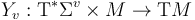 is a vector-field-valued 1-form on
  that is chosen compatibly with the fixed Hamiltonian perturbations as follows:
On the thin part ![\iota _{e}^{v}:[0,\infty )\times [0,1]\hookrightarrow \Sigma ^{v}](/images/math/d/1/1/d1100c1e7510c1014aac509f6b8fd6de.png) near each puncture
near each puncture  we have
 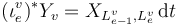 .
.
In particular, this convention together with our symmetric choice of Hamiltonian perturbations  forces the vector-field-valued 1-form on
 ![\Sigma ^{v}\simeq \mathbb{R} \times [0,1]](/images/math/5/6/a/56a3486ce4c38533929719c2fae3d318.png) in case
in case  to be
to be  -invariant,
  if
if  are the Lagrangian labels for the boundary components
  .
.
Here and in the following we denote  in case
  , so that
  in case
  .
.
The Hamiltonian perturbations  should be cut off to vanish outside of the thin parts of the domains
  . However, there may be thin parts of a surface that are not neighborhoods of a puncture. On these, we must choose the Hamiltonian-vector-field-valued one-form compatible with gluing as in [Seidel book].
For example, in the neighbourhood of a tree with an edge between main vertices, there are trees in which this edge is removed, the two vertices are replaced by a single vertex
. However, there may be thin parts of a surface that are not neighborhoods of a puncture. On these, we must choose the Hamiltonian-vector-field-valued one-form compatible with gluing as in [Seidel book].
For example, in the neighbourhood of a tree with an edge between main vertices, there are trees in which this edge is removed, the two vertices are replaced by a single vertex  , and the surfaces
  are replaced by a single glued surface
 for
for  . Compatibility with gluing requires that the Hamiltonian perturbation on these glued surfaces is also given by a gluing construction for Hamiltonians
  (in which the two perturbations
  agree and hence can be matched over a long neck
 ![[-R,R]\times [0,1]\subset \Sigma _{{v\#w}}](/images/math/7/c/1/7c10420071147771af7f4f746f0fc075.png) ).
).
- The Lagrangian boundary conditions are
 ; more precisely this requires
  for each adjacent edge
  .
. - The finite energy condition is
 .
. - The matching conditions for sphere bubble trees are
 for each main vertex and sphere bubble tree attaching point
  .
. - Finite energy together with the (perturbed) Cauchy-Riemann equation implies uniform convergence of
 near each puncture , and the limits are required to satisfy the following matching conditions:
- For edges whose Lagrangian boundary conditions agree, the map extends smoothly to the puncture , and its value is required to match with the evaluation of the Morse trajectory
 associated to the edge
  , that is
  for
for  .
. - For edges with different Lagrangian boundary conditions
 , the map
 ![u_{e}^{v}:=(\iota _{e}^{v})^{*}u_{v}:(-\infty ,0)\times [0,1]\to M](/images/math/6/3/7/63792330def3bf1b30267f5afb4d519f.png) has a uniform limit
has a uniform limit  for some
  , and this limit intersection point is required to match with the value of the constant 'Morse trajectory'
  associated to the edge , that is
  .
.
- For edges
8. The generalized pseudoholomorphic polygon is stable
in the sense that
any main vertex whose map has zero energy  has enough special points to have trivial isotropy, that is the number of boundary marked points
  plus twice the number of interior marked points
  is at least 3.
Finally, two generalized pseudoholomorphic polygons are equivalent  if
if
there is a tree isomorphism  and a tuple of disk biholomorphisms
  which preserve the tree, Morse trajectories, marked points, and pseudoholomorphic curves in the sense that
-
 preserves the tree structure and order of edges;
  for every
  ;
;-
 for every and adjacent edge ;
 -
 for every ;
 -
 for every and ;
 - the pseudoholomorphic maps are related by reparametrization,
 for every .
Warning: Our directional conventions differ somewhat from [Seidel book] and [J.Li thesis] as follows:
Unlike both references, we orient edges towards the root, in order to obtain a more natural interpretation of the leaves as incoming vertices as in [J.Li thesis], but unlike [Seidel book] which uses the language of 1 incoming striplike end and  outgoing striplike ends.
Since we also insist on ordering the marked points counter-clockwise on the boundary of the disk, we then have to work with positive striplike ends
outgoing striplike ends.
Since we also insist on ordering the marked points counter-clockwise on the boundary of the disk, we then have to work with positive striplike ends ![[0,\infty )\times [0,1]\hookrightarrow \Sigma ^{v}](/images/math/b/e/c/bec1bfe842c6b1916c804663467dcec7.png) near each marked point for an incoming edge
near each marked point for an incoming edge  to make sure that the boundary components are labeled in order:
  with
with  , and
, and  with
with  .
Analogously, a negative striplike end
.
Analogously, a negative striplike end ![(-\infty ,0]\times [0,1]\hookrightarrow \Sigma ^{v}](/images/math/c/7/3/c732b45e4625a7ffd19f60df1348fade.png) near the marked point
near the marked point  for the outgoing edge labels with
  and with
  .
.
This amounts to working on Floer cohomology in the sense that for e.g.  the output of the differential
  includes a sum over (amongst other more complicated trees) pseudoholomorphic strips
 ![b=[u:\mathbb{R} \times [0,1]\to M]](/images/math/d/9/6/d96a1d9a44f24bab4af54724bdfa170d.png) with fixed positive limit
with fixed positive limit  .
.
If no Hamiltonian perturbations are involved in the construction of a moduli space of generalized pseudoholomorphic polygons - i.e. if for each pair  the Lagrangians are either identical or transverse
  - then the symplectic area function on the moduli space is defined by
![\omega :\overline {\mathcal {M}}(x_{0};x_{1},\ldots ,x_{d})\to \mathbb{R} ,\quad b={\bigl [}T,\underline {\gamma },\underline {z},\underline {w},\underline {\beta },\underline {u}{\bigr ]}\mapsto \omega (b):=\sum _{{v\in V^{m}}}\textstyle \int _{{\Sigma _{v}}}u_{v}^{*}\omega \;+\;\sum _{{\beta _{w}\in \underline {\beta }}}\omega (\beta _{w})=\langle [\omega ],[b]\rangle ,](/images/math/a/3/1/a3115e83f279a76a70eaf2f248d977cd.png)
which - since  only depends on the total homology class of the generalized polygon
![[b]:=\sum _{{v\in V}}(\overline {u}_{v})_{*}[D]+\sum _{{\beta _{w}\in \underline {\beta }}}[\beta _{w}]\;\in \;H_{2}(M;L_{0}\cup L_{1}\ldots \cup L_{d}).](/images/math/3/2/1/321a107845d6cd857b754c4884454f7a.png)
Here  is defined by unique continuous continuation to the punctures at which or
  .
.
Differential Geometric TODO:
In the presence of Hamiltonian perturbations, the definition of the symplectic area function needs to be adjusted to match with the symplectic action functional on the Floer complexes and satisfy some properties (which also need to be proven in the unperturbed case):
-
 is invariant under deformations with fixed limits (used in proof of A-infty relations and invariance);
 - a bound on needs to imply Gromov-compactness ... which requires an area-energy identity for J-curves, but we are allowed (bounded!) error terms from e.g. Hamiltonian perturbations;
- invariance proofs arguing with 'upper triangular form' require contributions to
 to be of positive symplectic area, or constant strips/disks for zero symplectic area;
 - to work with the Novikov ring, rather than field, the symplectic area needs to be nonnegative for all polygons (not just the strips and other contributions to for which this is automatic). It *might* be possible to achieve this by remembering that the Hamilton functions for each pair of Lagrangians are only fixed up to a constant (not see in the Hamiltonian vector field or time-1-flow), so when constructing the Hamiltonian perturbation vector fields over Deligne-Mumford spaces, it might be possible to shift e.g. the outgoing Hamiltonian in such a way that the vector field can be constructed with 'curvature terms of the correct sign'.
Sphere bubble trees
The sphere bubble trees that are relevant to the compactification of the moduli spaces of pseudoholomorphic polygons are genus zero stable maps with one marked point, as described in e.g. [Chapter 5, McDuff-Salamon].
For a fixed almost complex structure  , we can use the combinatorial simplification of working with a single marked point to construct the moduli space of sphere bubble trees as

where
1. is a tree with sets of vertices  and edges , and a distinguished root vertex , which we use to orient all edges towards the root.
2.  is a tuple of marked points on the spherical domains
  ,
,
indexed by the edges of , and including a special root marked point as follows:
- For each vertex
 the tuple of mutually disjoint marked points
  is indexed by the edges
  adjacent to .
 - For the root vertex
 the tuple of mutually disjoint marked points
  is also indexed by the edges adjacent to , but is also required to be disjoint from the fixed marked point
  .
. - The marked points, except for
 , can also be denoted as and by the edges .
3.  is a tuple of pseudoholomorphic spheres for each vertex,
that is each is labeled by a smooth map  satisfying
Cauchy-Riemann equation, finite energy, and matching conditions as follows:
satisfying
Cauchy-Riemann equation, finite energy, and matching conditions as follows:
- The Cauchy-Riemann equation is
 .
. - The finite energy condition is
 .
. - The matching conditions are
 for each edge .
4. The sphere bubble tree is stable
in the sense that
any vertex whose map has zero energy (which is equivalent to being constant) has valence  . Here the marked point counts as one towards the valence
  of the root vertex; in other words the root vertex can be constant with just two adjacent edges.
Finally, two sphere bubble trees are equivalent  if
if
there is a tree isomorphism and a tuple of sphere biholomorphisms  which preserve the tree, marked points, and pseudoholomorphic curves in the sense that
- preserves the tree structure, in particular maps the root to the root
 ;
; -
 and for every and adjacent edge ;
 - the pseudoholomorphic spheres are related by reparametrization, for every .