Moduli spaces of pseudoholomorphic polygons

table of contents

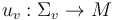
To construct the moduli spaces from which the composition maps are defined we fix an auxiliary almost complex structure $J:TM\to TM$ which is compatible with the symplectic structure in the sense that $\omega (\cdot ,J\cdot )$ defines a metric on $M$. (Unless otherwise specified, we will use this metric in all following constructions.)

Then given Lagrangians $L_{0},\ldots ,L_{d}\subset M$ and generators $x_{0}\in {\text{Crit}}(L_{0},L_{d}),x_{1}\in {\text{Crit}}(L_{0},L_{1}),\ldots ,x_{d}\in {\text{Crit}}(L_{{d-1}},L_{d})$ of their morphism spaces, we need to specify the Gromov-compactified moduli space $\overline {\mathcal {M}}(x_{0};x_{1},\ldots ,x_{d})$. (Here and throughout, we will call a moduli space Gromov-compact if its subsets of bounded symplectic area are compact in the Gromov topology.) We will do this by combining two special cases which we discuss first.

Pseudoholomorphic polygons for pairwise transverse Lagrangians

If each consecutive pair of Lagrangians is transverse, $L_{0}\pitchfork L_{1},L_{1}\pitchfork L_{2},\ldots ,L_{{d-1}}\pitchfork L_{d},L_{d}\pitchfork L_{0}$, then our construction is based on pseudoholomorphic polygons

$u:\Sigma \to M,\qquad u((\partial \Sigma )_{i})\subset L_{i},\qquad \overline \partial _{J}u=0,$

where $\Sigma =\Sigma _{{\underline {z}}}:=D\setminus \{z_{0},\ldots ,z_{d}\}$ is a disk with $d+1$ boundary punctures in counter-clockwise order $z_{0},\ldots ,z_{d}\subset \partial D$, and $(\partial \Sigma )_{i}$ denotes the boundary component between $z_{i},z_{{i+1}}$ (resp. between $z_{{d}},z_{0}$ for i=d). More precisely, we construct the (uncompactified) moduli spaces of pseudoholomorphic polygons for any tuple $x_{i}\in L_{i}\cap L_{{i+1}}$ for $i=0,\ldots ,d$ as in [Seidel book]:

${\mathcal {M}}(x_{0};x_{1},\ldots ,x_{d}):={\bigl \{}(\underline {z},u)\,{\big |}\,{\text{1. - 3.}}{\bigr \}}/\sim$

where

1. $\underline {z}=(z_{0},z_{1},\ldots ,z_{d})\subset \partial D$ is a tuple of pairwise disjoint marked points on the boundary of a disk, in counter-clockwise order.
2. $u:\Sigma _{{\underline {z}}}\to M$ is a smooth map satisfying
   • the Cauchy-Riemann equation $\overline \partial _{J}u=0$,
   • Lagrangian boundary conditions $u((\partial \Sigma )_{i})\subset L_{i}$,
   • the finite energy condition $\textstyle \int _{{\Sigma }}u^{*}\omega <\infty$,
   • the limit conditions $\lim _{{z\to z_{i}}}u(z)=x_{i}$ for $i=0,1,\ldots ,d$.
3. The pseudoholomorphic polygon $(\underline {z},u)$ is stable in the sense that the map $u:\Sigma _{{\underline {z}}}\to M$ is nonconstant if the number of marked points is $d+1<3$.

Here two pseudoholomorphic polygons are equivalent $(\underline {z},u)\sim (\underline {z}',u')$ if there is a disk automorphism $\psi :D\to D$ that preserves the complex structure on $D$, the marked points $\psi (z_{i})=z'_{i}$, and relates the pseudoholomorphic polygons by reparametrization, $u=u'\circ \psi$.

---

The case $d=0$ is not considered in this part of the moduli space setup since $L_{0},L_{d}=L_{0}$ are never transverse. However, it might appear in the construction of homotopy units?

The domains of the pseudoholomorphic polygons are strips for $d=1$ and represent elements in a Deligne-Mumford space for $d\geq 2$ as follows:

For $d=1$, the twice punctured disks are all biholomorphic to the strip $\Sigma _{{\{z_{0},z_{1}\}}}\simeq \mathbb{R} \times [0,1]$, so that we could equivalently set up the moduli spaces ${\mathcal {M}}(x_{0};x_{1})$ by fixing the domain $\Sigma _{{d=1}}:=\mathbb{R} \times [0,1]$ and defining the equivalence relation $\sim$ only in terms of the shift action $u(s,t)\mapsto u(\tau +s,t)$ of $\tau \in \mathbb{R}$. This is the only case in which the stability condition is nontrivial: It requires the maps $u:\mathbb{R} \times [0,1]\to M$ to be nonconstant.

For $d\geq 2$, the moduli space of domains

${\mathcal {M}}_{{d+1}}:={\frac {{\bigl \{}\Sigma _{{\underline {z}}}\,{\big |}\,\underline {z}=\{z_{0},\ldots ,z_{d}\}\in \partial D\;{\text{pairwise disjoint}}{\bigr \}}}{\Sigma _{{\underline {z}}}\sim \Sigma _{{\underline {z}'}}\;{\text{iff}}\;\exists \psi :\Sigma _{{\underline {z}}}\to \Sigma _{{\underline {z}'}},\;\psi ^{*}i=i}}$

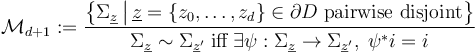
can be compactified to form the Deligne-Mumford space $\overline {\mathcal {M}}_{{d+1}}$, whose boundary and corner strata can be represented by trees of polygonal domains $(\Sigma _{v})_{{v\in V}}$ with each edge $e=(v,w)$ represented by two punctures $z_{e}^{-}\in \Sigma _{v}$ and $z_{e}^{+}\in \Sigma _{w}$. The thin neighbourhoods of these punctures are biholomorphic to half-strips, and a neighbourhood of a tree of polygonal domains is obtained by gluing the domains together at the pairs of strip-like ends represented by the edges.

All isotropy groups of this uncompactified moduli space ${\mathcal {M}}(x_{0};x_{1},\ldots ,x_{d})$ are trivial; that is any disk automorphism $\psi :D\to D$ that fixes $d+1\geq 1$ marked points $\psi (z_{i})=z_{i}$, and preserves a pseudoholomorphic map $u=u\circ \psi$ must be the identity $\psi ={{\rm {id}}}_{D}$.

Proof:

In case $d=2$ this follows directly from the marked points, since any Mobius transformation that fixes three points is the identity.

In case $d=1$ this requires both the stability and finite energy conditions: The group of automorphisms that fix two marked points - i.e. the automorphisms of the strip - are shifts by $\mathbb{R}$. On the other hand, any J-holomorphic map $u:\mathbb{R} \times [0,1]\to M$ has nonnegative energy density $u^{*}\omega ={\bigl (}|\partial _{s}u|^{2}+|\partial _{t}u|^{2}{\bigr )}ds\wedge dt$ with $|\partial _{s}u|=|\partial _{t}u|$. If we now had nontrivial isotropy, i.e. $u(\tau +s,t)=u(s,t)$ for some $\tau >0$ and a nonconstant map $u$, then there would exist $s_{0},t_{0}\in \mathbb{R} \times [0,1]$ with $|\partial _{s}u(s_{0},t_{0})|=|\partial _{t}u(s_{0},t_{0})|>0$ and thus $\textstyle \int _{{[s_{0}-{\frac {1}{2}}\tau ]\times [0,1]}}^{{[s_{0}+{\frac {1}{2}}\tau ]\times [0,1]}}u^{*}\omega >0$. However, this is in contradiction to $u$ having finite energy,

$\infty >\textstyle \int _{{\mathbb{R} \times [0,1]}}u^{*}\omega =\sum _{{k\in \mathbb{Z } }}\int _{{[s_{0}+(k-{\frac {1}{2}})\tau ]\times [0,1]}}^{{[s_{0}+(k+{\frac {1}{2}})\tau ]\times [0,1]}}u^{*}\omega =\sum _{{k\in \mathbb{Z } }}\int _{{[s_{0}-{\frac {1}{2}}\tau ]\times [0,1]}}^{{[s_{0}+{\frac {1}{2}}\tau ]\times [0,1]}}u^{*}\omega .$

Next, to construct the Gromov-compactified moduli spaces $\overline {\mathcal {M}}(x_{0};x_{1},\ldots ,x_{d})$ we have to add various strata to the moduli space of pseudoholomorphic polygons without breaking or nodes ${\mathcal {M}}(x_{0};x_{1},\ldots ,x_{d})$ defined above.

This is done precisely in the general construction below, but roughly requires to include breaking and bubbling, in particular

• include degenerate pseudoholomorphic polygons given by a tuple of pseudoholomorphic maps $u_{v}:\Sigma _{v}\to M$ whose domain is a nontrivial tree of domains $[(\Sigma _{v})_{{v\in V}},(z_{e}^{\pm })_{{e\in E}}]\in \overline {\mathcal {M}}_{{d+1}}$;
• allow for Floer breaking at each puncture of the domains $\Sigma _{v}$, i.e. a finite string of pseudoholomorphic strips in ${\mathcal {M}}(x;x'),{\mathcal {M}}(x';x''),\ldots ,{\mathcal {M}}(x^{{(k)}};x_{i})$;
• allow for disk bubbling at any boundary point of the above domains, i.e. a tree, each of whose vertices is represented by a pseudoholomorphic disk, with edges representing nodes - given by marked points on different disks at which the maps satisfy a matching condition;
• allow for sphere bubbling at any (boundary or interior) point of each of the above domains, i.e. a tree, each of whose vertices is represented by a pseudoholomorphic sphere, with edges representing nodes - given by marked points on different spheres at which the maps satisfy a matching condition.

We will see that sphere bubbling does not contribute to the boundary stratification of these moduli spaces, so that the boundary stratification and thus the algebraic structure arising from these moduli spaces is induced by Floer breaking and disk bubbling. (On the other hand, sphere bubbling will be the only source of nontrivial isotropy.) The boundary strata arising from Floer breaking are fiber products of other moduli spaces of pseudoholomorphic polygons over finite sets of Lagrangian intersection points, which indicates an algebraic composition in this finitely generated Floer chain complex.

Disk bubbling, on the other hand, in the present setting yields boundary strata that are fiber products over the Lagrangian submanifold specified by the boundary condition, which is problematic for a combination of algebra and regularity reasons.

The corresponding algebraic composition requires a push-pull construction on some space of chains, currents, or differential forms on the Lagrangian. However, such constructions require transversality of the chains to the evaluation maps from the regularized moduli spaces, so that a rigorous construction of the $A_{\infty }$-structure in this setting - as in the approach by Fukaya et al - requires a complicated infinite iteration.

We will resolve this issue as in [J.Li thesis] by following another earlier proposal by Fukaya-Oh to allow disks to flow apart along a Morse trajectory, thus yielding disk trees which are constructed next - still ignoring sphere bubbling - before we put everything together to a general construction of the Gromov-compactified moduli space.

Pseudoholomorphic disk trees for a fixed Lagrangian

If the Lagrangians are all the same, $L_{0}=L_{1}=\ldots =L_{d}=:L$, then our construction is based on pseudoholomorphic disks

$u:D\to M,\qquad u(\partial D)\subset L,\qquad \overline \partial _{J}u=0.$

Such disks (modulo reparametrization by automorphisms of the disk) also arise from Gromov-compactifying other moduli spaces of pseudoholomorphic curves in which energy concentrates at a boundary point. To capture this bubbling algebraically, we work throughout with the Morse function $f:L\to \mathbb{R}$ chosen in the setup of the morphism space 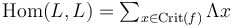${\text{Hom}}(L,L)=\textstyle \sum _{{x\in {\text{Crit}}(f)}}\Lambda x$. We also choose a metric on $L$ so that the gradient vector field $\nabla f$ satisfies the Morse-Smale conditions and an additional technical assumption in [1] which guarantees a natural smooth manifold-with-boundary-and-corners structure on the compactified Morse trajectory spaces $\overline {\mathcal {M}}(L,L),\overline {\mathcal {M}}(p^{-},L),\overline {\mathcal {M}}(L,p^{+}),\overline {\mathcal {M}}(p^{-},p^{+})$ for $p^{\pm }\in {\text{Crit}}(f)$. This smooth structure is essentially induced by the requirement that the evaluation maps at positive and negative ends ${{\rm {ev^{\pm }}}}:\overline {\mathcal {M}}(\ldots )\to L$ are smooth. With that data and the fixed almost complex structure $J$ we can construct the moduli spaces of pseudoholomorphic disk trees for any tuple 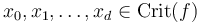$x_{0},x_{1},\ldots ,x_{d}\in {{\rm {Crit}}}(f)$ as in JL:

${\mathcal {M}}(x_{0};x_{1},\ldots ,x_{d}):={\bigl \{}(T,\underline {\gamma },\underline {z},\underline {u})\,{\big |}\,{\text{1. - 5.}}{\bigr \}}/\sim$

where

1. $T$ is an ordered tree with sets of vertices $V=V^{m}\cup V^{c}$ and edges $E$,

equipped with orientations towards the root, orderings of incoming edges, and a partition into main and critical (leaf and root) vertices as follows:

• The edges $E\subset V\times V\setminus \Delta _{V}$ are oriented towards the root vertex $v_{0}\in V$ of the tree, i.e. for $e=(v,w)\in E$ the outgoing vertex $w$ is still connected to the root after removing $e$. Thus each vertex $v\in V$ has a unique outgoing edge $e_{v}^{0}=(v,\;\cdot \;)\in E$ (except for the root vertex which has no outgoing edge) and a (possibly empty) set of incoming edges $E_{v}^{{{\rm {in}}}}=\{e=(\;\cdot \;,v)\in E\}$. Moreover, the set of incoming edges is ordered, $E_{v}^{{{\rm {in}}}}=\{e_{v}^{1},\ldots ,e_{v}^{{|v|-1}}\}$ with $|v|$ denoting the valence - number of attached edges - of $v$.
• The set of vertices is partitioned $V=V^{m}\sqcup V^{c}$ into the sets of main vertices $V^{m}$ and the set of critical vertices $V^{c}=\{v_{0}^{c},v_{1}^{c},\ldots v_{d}^{c}\}$. The latter is ordered to start with the root $v_{0}^{c}=v_{0}$, which is required to have a single edge $\{e_{{v_{0}}}^{1}\}=E_{{v_{0}}}^{{{\rm {in}}}}$, and then contains d leaves $v_{i}^{c}$ of the tree (i.e. with $E_{{v_{i}^{c}}}^{{{\rm {in}}}}=\emptyset$), with order induced by the orientation and order of the edges (with the root being the minimal vertex).

2. $\underline {\gamma }=(\underline {\gamma }_{e})_{{e\in E}}$ is a tuple of generalized Morse trajectories for each edge

in the following compactified Morse trajectory spaces:

• $\underline {\gamma }_{e}\in \overline {\mathcal {M}}(x_{i},x_{j})$ for any edge $e=(v_{i}^{c},v_{j}^{c})$ between critical vertices;
• $\underline {\gamma }_{e}\in \overline {\mathcal {M}}(x_{i},L)$ for any edge $e=(v_{i}^{c},w)$ from a critical vertex $v_{i}^{c}$ to a main vertex $w\in V^{m}$;
• $\underline {\gamma }_{e}\in \overline {\mathcal {M}}(L,x_{j})$ for any edge $e=(v,v_{j}^{c})$ from a main vertex $v\in V^{m}$ to a critical vertex $v_{j}^{c}$;
• $\underline {\gamma }_{e}\in \overline {\mathcal {M}}(L,L)$ for any edge $e=(v,w)$ between main vertices $v,w\in V^{m}$.

3. $\underline {z}=(\underline {z}_{v})_{{v\in V^{m}}}$ is a tuple of boundary marked points for each main vertex

that are ordered counter-clockwise as follows:

• For each main vertex $v$ there are $|v|$ pairwise disjoint marked points $\underline {z}_{v}=(z_{e}^{v})_{{e\in \{e_{v}^{0}\}\cup E_{v}^{{{\rm {in}}}}}}\subset \partial D$ on the boundary of a disk.
• The order $\{e_{v}^{0}\}\cup E_{v}^{{{\rm {in}}}}=\{e_{v}^{0},e_{v}^{1},\ldots ,e_{v}^{{|v|-1}}\}$ of the edges corresponds to a counter-clockwise order of the marked points $z_{{e_{v}^{0}}}^{v},z_{{e_{v}^{1}}}^{v},\ldots ,z_{{e_{v}^{{|v|-1}}}}^{v}\in \partial D$.
• The marked points can also be denoted as $z_{e}^{-}=z_{e}^{v}$ and $z_{e}^{+}=z_{e}^{w}$ by the edges $e=(v,w)\in E$ for which $v\in V^{m}$ or $w\in V^{m}$.

4. $\underline {u}=(\underline {u}_{v})_{{v\in V^{m}}}$ is a tuple of pseudoholomorphic disks for each main vertex,

that is each $v\in V^{m}$ is labeled by a smooth map $u_{v}:D\to M$ satisfying Cauchy-Riemann equation, Lagrangian boundary condition, finite energy, and matching conditions as follows:

• The Cauchy-Riemann equation is $\overline \partial _{J}u_{v}=0$.
• The Lagrangian boundary condition is $u_{v}(\partial D)\subset L<\infty$.
• The finite energy condition is $\textstyle \int _{D}u_{v}^{*}\omega <\infty$.
• The pseudholomorphic disks can also be indexed as $u_{e}^{-}=u_{v}$ and $u_{e}^{+}=u_{w}$ by the edges $e=(v,w)\in E$ for which $v\in V^{m}$ or $w\in V^{m}$. In that notation, they satisfy the matching conditions with the generalized Morse trajectories $u_{e}^{\pm }(z_{e}^{\pm })={{\rm {ev}}}^{\pm }(\underline {\gamma }_{e})$ whenever $v_{e}^{\pm }\in V^{m}$.

5. The disk tree is stable

in the sense that

any main vertex $v\in V^{m}$ whose disk has zero energy $\textstyle \int u_{v}^{*}\omega =0$ (which is equivalent to $u_{v}$ being constant) has valence $|v|\geq 3$.

Finally, two pseudoholomorphic disk trees are equivalent $(T,\underline {\gamma },\underline {z},\underline {u})\sim (T',\underline {\gamma }',\underline {z}',\underline {u}')$ if

there is a tree isomorphism $\zeta :T\to T'$ and a tuple of disk automorphisms $(\psi _{v}:D\to D)_{{v\in V^{m}}}$ which preserving the tree, complex structure, Morse trajectories, marked points, and pseudoholomorphic curves in the sense that

• $\zeta$ preserves the tree structure and order of edges;
• $\psi ^{*}i=i$, where $i:TD\to TD$ denotes the complex structure on $D$;
• $\underline {\gamma }_{e}=\underline {\gamma }'_{{\zeta (e)}}$ for every $e\in E$;
• $\psi _{v}(z_{e}^{v})=z_{{\zeta (e)}}^{{'\;\zeta (v)}}$ for every $v\in V^{m}$ and adjacent edge $e\in E$;
• the pseudoholomorphic disks are related by reparametrization, $u_{v}=u'_{{\zeta (v)}}\circ \psi _{v}$ for every $v\in V^{m}$.

---

The domains of the disk trees are never stable for $d=0,1$, but need to be studied to construct the differential $\mu ^{1}$ on the Floer chain complex and the curvature term $\mu ^{0}$ that may obstruct $\mu ^{1}\circ \mu ^{1}=0$. For $d\geq 2$ the domains of the disk trees represent elements in a Deligne-Mumford space as follows:

Any equivalence class of disk trees $[(T,\underline {\gamma },\underline {z},\underline {u})]$ induces a domain tree $[(T',\underline {\ell },\underline {z})]$

by forgetting the Morse trajectories and pseudoholomorphic maps as follows:

1. The tree $T'$ is obtained from $T$ by replacing critical vertices and their outgoing edges by incoming semi-infinite edges of the new tree $T'$. We also replace the critical root vertex and its incoming edge by an outgoing semi-infinite edge of the new tree $T'$. The new tree $T'$ retains the orientations of edges and inherits an order of the edges from $T$. Its root is the unique main vertex from which there was an edge to the critical root vertex in $T$.
2. Every vertex $v\in V'=V^{m}$ of $T'$ then represents a disk domain $D_{v}=D$.
3. Every edge $e\in E'=E$ is labeled with the length $\ell _{e}:=\ell (\underline {\gamma }_{e})\in [0,\infty ]$ of the associated generalized Morse trajectory. For the semi-infinite edges, this length is automatically $\ell _{e}=\infty$ since the associated Morse trajectories are semi-infinite.
4. The domain for each vertex $v\in V'$ is marked by $|v|$ boundary points $\underline {z}_{v}=(z_{e}^{v})_{{e\in \{e_{v}^{0}\}\cup E_{v}^{{{\rm {in}}}}}}\subset \partial D_{v}$, ordered counter-clockwise.
5. Two such trees are equivalent $[(T,\underline {\ell },\underline {z})]\sim [(T',\underline {\ell }',\underline {z}')]$ if there is a tree isomorphism $\zeta :T\to T'$ and a tuple of disk automorphisms $(\psi _{v}:D\to D)_{{v\in V^{m}}}$ preserving the complex structure on $D$ such that $\zeta$ preserves the ordered tree structure and lengths $\ell _{e}=\ell '_{{\zeta (e)}}$ for every $e\in E$, and the marked points are preserved $\psi _{v}(z_{e}^{v})=z{'\;\zeta (v)}_{{\zeta (e)}}$ for every $v\in V^{m}$ and adjacent $e\in E$.

For $d\geq 2$, such a domain tree is called stable if every vertex has valence $|v|\geq 3$ - i.e. there are at least three marked points on each disk $D_{v}$. The domain trees for $d=0,1$ are never stable, but both cases need to be included in our moduli space constructions: The differential $\mu ^{1}$ on the Floer chain complex $Hom(L,L)=\textstyle \sum _{{x\in {{\rm {Crit}}}(f)}}\Lambda \;x$ is constructed by counting the elements of ${\mathcal {M}}(x_{0};x_{1})$. The curvature term $\mu ^{0}$, which is constructed from moduli spaces ${\mathcal {M}}(x_{0})$ with no incoming critical points, serves to algebraically encode disk bubbling in any moduli space involving a Lagrangian boundary condition on $L$.

For $d\geq 2$, while the above trees are not necessarily stable, they induce unique stable rooted metric ribbon trees $(T,\underline {\ell })$ in the sense of [Def.2.7, MW], by forgetting the marked points, forgetting every leaf of valence 1 and its outgoing edge, and replacing every vertex $v$ of valence 2 and its incoming and outgoing edges $(v^{-},v),(v,v^{+})$ by a single edge $(v^{-},v^{+})$ of length $\ell _{{(v^{-},v^{+})}}=\ell _{{(v^{-},v)}}+\ell _{{(v,v^{+})}}$. The space of such stable rooted metric ribbon trees - where a tree containing an edge of length $\ell _{e}=0$ is identified with the tree in which this edge and its adjacent vertices are replaced by a single vertex - is another topological representation of the Deligne Mumford space $\overline {\mathcal {M}}_{{d+1}}$, as discussed in [BV]. Its boundary strata are given by trees with interior edges of length $\ell _{e}=\infty$.

We now expect the boundary stratification of the moduli spaces of disk trees ${\mathcal {M}}(x_{0};x_{1},\ldots ,x_{d})$ - if/once regular - to arise exclusively from breaking of the Morse trajectories representing edges of the disk trees. This is made rigorous in [J.Li thesis] under the assumption that the almost complex structure $J$ can be chosen such that there exist no nonconstant $J$-holomorphic spheres in the symplectic manifold $M$. In that special case, all isotropy groups are trivial by [Prop.2.5, J.Li thesis]; that is any equivalence between a disk tree and itself, $(T,\underline {\gamma },\underline {z},\underline {u})\sim (T,\underline {\gamma },\underline {z},\underline {u})$, is given by the trivial tree isomorphism $\zeta :T\to T$, and the only disk automorphisms $(\psi _{v}:D\to D)_{{v\in V^{m}}}$ which preserve the marked points and pseudoholomorphic disk maps are the identity maps $\psi _{v}={{\rm {id}}}_{D}$. In this case, the moduli spaces of disk trees ${\mathcal {M}}(x_{0};x_{1},\ldots ,x_{d})$ are moreover Gromov-compact since sphere bubbling is ruled out and disk bubbling is captured by edges labeled with constant, zero length, Morse trajectories.

In general, we will Gromov-compactify ${\mathcal {M}}(x_{0};x_{1},\ldots ,x_{d})$ in the following general construction by allowing for sphere bubble trees developing at any (boundary or interior) point of each of the disk domains. This will also be a source of generally nontrivial isotropy.

General moduli space of pseudoholomorphic polygons

For the construction of a general $A_{\infty }$-composition map we are given $d+1\geq 1$ Lagrangians $L_{0},\ldots ,L_{d}\subset M$ and choices of Hamiltonian diffeomorphisms $\phi _{i}:=\phi _{{L_{{i-1}},L_{i}}}:M\to M$ such that $\phi _{i}(L_{{i-1}})\pitchfork L_{i}$, whenever $L_{{i-1}}\neq L_{i}$. (Here and in the following we will often index by $i\in \mathbb{Z } _{{d+1}}$, so in particular for $i=0$, unless $L_{d}=L_{0}$, we are given $\phi _{0}:=\phi _{{L_{d},L_{0}}}$ such that $\phi _{0}(L_{d})\pitchfork L_{0}$.) Then given generators $x_{0}\in {\text{Crit}}(L_{0},L_{d}),x_{1}\in {\text{Crit}}(L_{0},L_{1}),\ldots ,x_{d}\in {\text{Crit}}(L_{{d-1}},L_{d})$ of their morphism spaces, we construct the Gromov-compactified moduli space of pseudoholomorphic polygons by combining the two special cases above:

${\mathcal {M}}(x_{0};x_{1},\ldots ,x_{d}):={\bigl \{}(T,\underline {L},\underline {\gamma },\underline {z},\underline {u})\,{\big |}\,{\text{1. - 6.}}{\bigr \}}/\sim$

where

1. $T$ is an ordered tree with sets of vertices $V=V^{m}\cup V^{c}$ and edges $E$,

equipped with orientations towards the root, orderings of incoming edges, and a partition into main and critical (leaf and root) vertices as follows:

• The edges $E\subset V\times V\setminus \Delta _{V}$ are oriented towards the root vertex $v_{0}\in V$ of the tree, so that each vertex $v\in V$ has a unique outgoing edge $e_{v}^{0}=(v,\;\cdot \;)\in E$ (except for the root vertex which has no outgoing edge) and a (possibly empty) set of incoming edges $E_{v}^{{{\rm {in}}}}=\{e=(\;\cdot \;,v)\in E\}$.
• The set of incoming edges is ordered, $E_{v}^{{{\rm {in}}}}=\{e_{v}^{1},\ldots ,e_{v}^{{|v|-1}}\}$. This induces a cyclic order on the set of all edges $E_{v}:=\{e_{v}^{0},e_{v}^{1},\ldots ,e_{v}^{{|v|-1}}\}$ adjacent to $v$, by setting $e_{v}^{{|v|}}=e_{v}^{0}$, and we will denote consecutive edges in this order by $e=e_{v}^{i},e+1=e_{v}^{{i+1}}$. In particular this yields $e_{v}^{0}+i=e_{v}^{i}$.
• The set of vertices is partitioned $V=V^{m}\sqcup V^{c}$ into the sets of main vertices $V^{m}$ and critical vertices $V^{c}=\{v_{0}^{c},v_{1}^{c},\ldots v_{d}^{c}\}$. The latter is ordered to start with the root $v_{0}^{c}=v_{0}$ and then contains d leaves $v_{i}^{c}$ of the tree, with order induced by the orientation and order of the edges.
• The root vertex $v_{0}^{c}\in V^{c}$ has a single edge $\{e_{{v_{0}}}^{1}=(v,v_{0}^{c})\}=E_{{v_{0}}}^{{{\rm {in}}}}=E_{{v_{0}}}$, and this attaches to a main vertex $v\in V^{m}$ except for one special case: For $d=1$ and $L_{d}=L_{0}$ we allow the tree with a single edge $e=(v_{1}^{c},v_{0}^{c})$ between its two critical vertices $V=\{v_{0}^{c},v_{1}^{c}\}$.

2. $\underline {L}=(\underline {L}^{v})_{{v\in V^{m}}}$ is a tuple of Lagrangian labels

that label the boundary components of domains in overall counter-clockwise order $L_{0},\ldots ,L_{d}$ as follows:

• For each main vertex $v\in V^{m}$ the Lagrangian label $\underline {L}^{v}=(L_{e}^{v})_{{e\in E_{v}}}$ is a cyclic sequence of Lagrangians $L_{e}^{v}\in \{L_{0},\ldots ,L_{d}\}$ indexed by the adjacent edges $E_{v}$ (which will become the boundary condition on $(\partial \Sigma ^{v})_{e}$).
• For each edge $e=(v^{-},v^{+})\in E$ the Lagrangian labels satisfy a matching condition as follows:
  • The edge from a critical leaf $v^{-}=v_{i}^{c}\in V^{c}$ requires $L_{e}^{{v^{+}}}=L_{i},L_{{e-1}}^{{v^{+}}}=L_{{i-1}}$.
  • The edge to the critical root $v^{+}=v_{0}^{c}\in V^{c}$ requires $L_{e}^{{v^{-}}}=L_{0},L_{{e-1}}^{{v^{-}}}=L_{d}$.
  • Any edge between main vertices $v^{-},v^{+}\in V^{m}$ requires $L_{{e}}^{{v^{-}}}=L_{{e-1}}^{{v^{+}}}$ and $L_{{e-1}}^{{v^{-}}}=L_{{e}}^{{v^{+}}}$.

3. $\underline {\gamma }=(\underline {\gamma }_{e})_{{e\in E}}$ is a tuple of generalized Morse trajectories

in the following compactified Morse trajectory spaces:

• Any edge $e=(v_{i}^{c},w)$ from a critical leaf $v_{i}^{c}$ to a main vertex $w\in V^{m}$ is labeled by a half-infinite Morse trajectory $\underline {\gamma }_{e}\in \overline {\mathcal {M}}(x_{i},L_{i})$ if $L_{{i-1}}=L_{i}$, resp. by the constant $\underline {\gamma }_{e}\equiv x_{i}\in {{\rm {Crit}}}(L_{{i-1}},L_{i})$ in the discrete space $\phi _{i}(L_{{i-1}})\cap L_{i}$ if $L_{{i-1}}\neq L_{i}$.
• If the edge to the root $e=(v,v_{0}^{c})$ attaches to a main vertex $v\in V^{m}$ then it is labeled by a half-infinite Morse trajectory $\underline {\gamma }_{e}\in \overline {\mathcal {M}}(L_{0},x_{0})$ if $L_{d}=L_{0}$, resp. by the constant $\underline {\gamma }_{e}\equiv x_{0}\in {{\rm {Crit}}}(L_{d},L_{0})$ in the discrete space $\phi _{0}(L_{d})\cap L_{0}$ if $L_{d}\neq L_{0}$.
• An edge $e=(v_{i}^{c},v_{j}^{c})$ between critical vertices is labeled by an infinite Morse trajectory $\underline {\gamma }_{e}\in \overline {\mathcal {M}}(x_{i},x_{j})$ (this occurs only for $d=1$ with $L_{0}=L_{1}$ and the tree with one edge $e=(v_{1}^{c},v_{0}^{c})$).
• Any edge $e=(v,w)$ between main vertices $v,w\in V^{m}$ is labeled by a finite or infinite Morse trajectory $\underline {\gamma }_{e}\in \overline {\mathcal {M}}(L_{e}^{v},L_{e}^{v})$ in case $L_{e}^{v}=L_{{e-1}}^{v}$, resp. by a constant $\underline {\gamma }_{e}\equiv x_{e}\in {{\rm {Crit}}}(L_{{e-1}}^{v},L_{{e}}^{v})$ in the discrete space $\phi _{{L_{{e-1}}^{v},L_{{e}}^{v}}}(L_{{e-1}}^{v})\cap L_{e}^{v}$ in case $L_{e}^{v}\neq L_{{e-1}}^{w}$. (Recall the matching condition $L_{e}^{v}=L_{{e-1}}^{w}$ and $L_{{e-1}}^{v}=L_{e}^{w}$ from 2.)

4. $\underline {z}=(\underline {z}_{v})_{{v\in V^{m}}}$ is a tuple of boundary points

that are ordered counter-clockwise and associate complex domains $\Sigma ^{v}:=D\setminus \underline {z}_{v}$ to the vertices as follows:

• For each main vertex $v$ there are $|v|$ pairwise disjoint marked points $\underline {z}_{v}=(z_{e}^{v})_{{e\in E_{v}}}\subset \partial D$ on the boundary of a disk.
• The order $E_{v}=\{e_{v}^{0},e_{v}^{1},\ldots ,e_{v}^{{|v|-1}}\}$ of the edges corresponds to a counter-clockwise order of the marked points $z_{{e_{v}^{0}}}^{v},z_{{e_{v}^{1}}}^{v},\ldots ,z_{{e_{v}^{{|v|-1}}}}^{v}\in \partial D$.
• The marked points can also be denoted as $z_{e}^{-}=z_{e}^{v}$ and $z_{e}^{+}=z_{e}^{w}$ by the edges $e=(v,w)\in E$ for which $v\in V^{m}$ or $w\in V^{m}$
• To each main vertex $v\in V^{m}$ we associate the punctured disk $\Sigma ^{v}:=D\setminus \underline {z}_{v}$. Then the marked points $\underline {z}^{v}=(z_{e}^{v})_{{e\in E_{v}}}\subset \partial D$ partition the boundary into $|v|$ connected components $\partial \Sigma ^{v}=\textstyle \sqcup _{{e\in E_{v}}}(\partial \Sigma ^{v})_{e}$ such that the closure of each component $(\partial \Sigma ^{v})_{e}$ contains the marked points $z_{e}^{v},z_{{e+1}}^{v}$.

5. $\underline {u}=(\underline {u}_{v})_{{v\in V^{m}}}$ is a tuple of pseudoholomorphic maps for each main vertex,

that is each $v\in V^{m}$ is labeled by a smooth map $u_{v}:\Sigma ^{v}\to M$ satisfying Cauchy-Riemann equation, Lagrangian boundary conditions, finite energy, and matching conditions as follows:

• The Cauchy-Riemann equation is $\overline \partial _{J}u_{v}=0$.

HAMILTONIAN PERTURBATION

• The Lagrangian boundary conditions are $u_{v}(\partial \Sigma ^{v})\subset \underline {L}^{v}$; more precisely this requires $u_{v}{\bigl (}(\partial \Sigma ^{v})_{e}{\bigr )}\subset L_{e}^{v}$ for each adjacent edge $e\in E_{v}$.
• The finite energy condition is $\textstyle \int _{{\Sigma ^{v}}}u_{v}^{*}\omega <\infty$.

This implies smooth extension of $u_{v}$ to any puncture $z_{e}^{v}$ whenever the Lagrangian boundary conditions $L_{{e-1}}^{v}=L_{e}^{v}$ agree.

• The pseudholomorphic maps can also be indexed as $u_{e}^{-}=u_{v}$ and $u_{e}^{+}=u_{w}$ by the edges $e=(v,w)\in E$ for which $v\in V^{m}$ or $w\in V^{m}$. In that notation, they satisfy the matching conditions

$u_{e}^{\pm }(z_{e}^{\pm })={{\rm {ev}}}^{\pm }(\underline {\gamma }_{e})$ whenever $v_{e}^{\pm }\in V^{m}$.

6. The disk tree is stable

in the sense that

any main vertex $v\in V^{m}$ whose disk has zero energy $\textstyle \int u_{v}^{*}\omega =0$ (which is equivalent to $u_{v}$ being constant) has valence $|v|\geq 3$.

Finally, two pseudoholomorphic disk trees are equivalent $(T,\underline {\gamma },\underline {z},\underline {u})\sim (T',\underline {\gamma }',\underline {z}',\underline {u}')$ if

there is a tree isomorphism $\zeta :T\to T'$ and a tuple of disk automorphisms $(\psi _{v}:D\to D)_{{v\in V^{m}}}$ which preserving the tree, complex structure, Morse trajectories, marked points, and pseudoholomorphic curves in the sense that

• $\zeta$ preserves the tree structure and order of edges;
• $\psi ^{*}i=i$, where $i:TD\to TD$ denotes the complex structure on $D$;
• $\underline {\gamma }_{e}=\underline {\gamma }'_{{\zeta (e)}}$ for every $e\in E$;
• $\psi _{v}(z_{e}^{v})=z_{{\zeta (e)}}^{{'\;\zeta (v)}}$ for every $v\in V^{m}$ and adjacent edge $e\in E$;
• the pseudoholomorphic disks are related by reparametrization, $u_{v}=u'_{{\zeta (v)}}\circ \psi _{v}$ for every $v\in V^{m}$.

Make up for differences in Hamiltonian symplectomorphisms applied to each Lagrangian by a domain-dependent Hamiltonian perturbation to the Cauchy-Riemann equation

NOTE: when degenerating polygons to create a strip with $L_{i}=L_{j}$ boundary conditions, will need to transfer from Morse-Bott breaking to boundary node

Finally, the symplectic area function $\omega :\overline {\mathcal {M}}(x_{0};x_{1},\ldots ,x_{d})\to \mathbb{R}$ in each case is given by TODO

Fredholm index ${\mathcal {M}}^{k}(\ldots )=\{b\in {\mathcal {M}}(\ldots )\,|\,IND...=k\}$