Moduli spaces of pseudoholomorphic polygons

table of contents

To construct the moduli spaces from which the composition maps are defined we fix an auxiliary almost complex structure $J:TM\to TM$ which is compatible with the symplectic structure in the sense that $\omega (\cdot ,J\cdot )$ defines a metric on $M$. (Unless otherwise specified, we will use this metric in all following constructions.) Then given Lagrangians $L_{0},\ldots ,L_{d}\subset M$ and generators $x_{0}\in {\text{Crit}}(L_{0},L_{d}),x_{1}\in {\text{Crit}}(L_{0},L_{1}),\ldots ,x_{d}\in {\text{Crit}}(L_{{d-1}},L_{d})$ of their morphism spaces, we need to specify the (compactified) moduli space $\overline {\mathcal {M}}(x_{0};x_{1},\ldots ,x_{d})$. We will do this by combining two special cases which we discuss first.

Pseudoholomorphic polygons for pairwise transverse Lagrangians

If each consecutive pair of Lagrangians is transverse, i.e. $L_{0}\pitchfork L_{1},L_{1}\pitchfork L_{2},\ldots ,L_{{d-1}}\pitchfork L_{d},L_{d}\pitchfork L_{0}$, then our construction is based on pseudoholomorphic polygons

$u:\Sigma \to M,\qquad u((\partial \Sigma )_{i})\subset L_{i},\qquad \overline \partial _{J}u=0,$

where $\Sigma =\Sigma _{{\underline {z}}}:=D\setminus \{z_{0},\ldots ,z_{d}\}$ is a disk with $d+1$ boundary punctures in counter-clockwise order $z_{0},\ldots ,z_{d}\subset \partial D$, and $(\partial \Sigma )_{i}$ denotes the boundary component between $z_{i},z_{{i+1}}$ (resp. between $z_{{d}},z_{0}$ for i=d). More precisely, we construct the (uncompactified) moduli spaces of pseudoholomorphic polygons for any tuple $x_{i}\in L_{i}\cap L_{{i+1}}$ for $i=0,\ldots ,d$ as in [S]:

${\mathcal {M}}(x_{0};x_{1},\ldots ,x_{d}):={\bigl \{}(\underline {z},u)\,{\big |}\,{\text{1. - 2.}}{\bigr \}}/\sim$

where

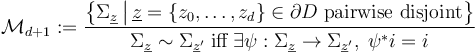
1. $\underline {z}=(z_{0},z_{1},\ldots ,z_{d})\subset \partial D$ is a tuple of pairwise disjoint marked points on the boundary of a disk, in counter-clockwise order.
2. $u:\Sigma _{{\underline {z}}}\to M$ is a smooth map satisfying
   • the Cauchy-Riemann equation $\overline \partial _{J}u=0$,
   • Lagrangian boundary conditions $u((\partial \Sigma )_{i})\subset L_{i}<\infty$,
   • the finite energy condition $\textstyle \int _{{\Sigma }}u^{*}\omega <\infty$,
   • the limit conditions $\lim _{{z\to z_{i}}}u(z)=x_{i}$ for $i=0,1,\ldots ,d$.

Here two pseudoholomorphic polygons are equivalent $(\underline {z},u)\sim (\underline {z}',u')$ if there is a disk automorphism $\psi :D\to D$ that preserves the complex structure on $D$, the marked points $\psi (\underline {z})=\underline {z}'$, and relates the pseudoholomorphic polygons by reparametrization, $u=u'\circ \psi$.

For $d=1$, the twice punctured disks are all biholomorphic to the strip $\Sigma _{{\{z_{0},z_{1}\}}}\simeq \mathbb{R} \times [0,1]$, so that we could equivalently set up the moduli spaces ${\mathcal {M}}(x_{0};x_{1})$ by fixing the domain $\Sigma _{{d=1}}:=\mathbb{R} \times [0,1]$ and defining the equivalence relation $\sim$ only in terms of the shift action $u(s,t)\mapsto u(\tau +s,t)$ of $\tau \in \mathbb{R}$.

For $d\geq 2$, the moduli space of domains

${\mathcal {M}}_{{d+1}}:={\frac {{\bigl \{}\Sigma _{{\underline {z}}}\,{\big |}\,\underline {z}=\{z_{0},\ldots ,z_{d}\}\in \partial D\;{\text{pairwise disjoint}}{\bigr \}}}{\Sigma _{{\underline {z}}}\sim \Sigma _{{\underline {z}'}}\;{\text{iff}}\;\exists \psi :\Sigma _{{\underline {z}}}\to \Sigma _{{\underline {z}'}},\;\psi ^{*}i=i}}$

can be compactified to form the Deligne-Mumford space $\overline {\mathcal {DM}}_{{d+1}}$, whose boundary and corner strata can be represented by trees of polygonal domains $(\Sigma _{v})_{{v\in V}}$ with each edge $e=(v,w)$ represented by two punctures $z_{e}^{-}\in \Sigma _{v}$ and $z_{e}^{+}\in \Sigma _{w}$. The thin neighbourhoods of these punctures are biholomorphic to half-strips, and then a neighbourhood of a tree of polygonal domains is obtained by gluing the domains together at the pairs of strip-like ends represented by the edges.

compactified moduli spaces

$\overline {\mathcal {M}}(x_{0};x_{1},\ldots ,x_{d})$

Pseudoholomorphic disk trees for a fixed Lagrangian

If the Lagrangians are all the same, $L_{0}=L_{1}=\ldots =L_{d}=:L$, then our construction is based on pseudoholomorphic disks

$u:D\to M,\qquad u(\partial D)\subset L,\qquad \overline \partial _{J}u=0.$

For a sequence of such maps (modulo reparametrization by automorphisms of the disk), energy concentration at a boundary point is usually captured in terms of a disk bubble attached via a boundary node. This yields to a compactification of the moduli space of pseudoholomorphic disks modulo reparametrization that is given by adding boundary strata consisting of fiber products of moduli spaces of disks. One could - as in the approach by Fukaya et al - regularize such a space and then interpret disk bubbling as contribution to $\widehat \mu \circ \widehat \mu$ - where the composition is via a push-pull construction on some space of chains, currents, or differential forms on the Lagrangian. However, such push-pull constructions require transversality of the chains to the evaluation maps from the regularized moduli spaces, so that a rigorous construction of the $A_{\infty }$-structure in this setting requires a complicated infinite iteration.

We will resolve this issue as in [JL] by following another earlier proposal by Fukaya-Oh to allow disks to flow apart along a Morse trajectory. Here we work throughout with the Morse function $f:L\to \mathbb{R}$ chosen in the setup of the morphism space ${\text{Hom}}(L,L)=\textstyle \sum _{{x\in {\text{Crit}}(f)}}\Lambda x$. We also choose a metric on $L$ so that the gradient vector field $\nabla f$ satisfies the Morse-Smale conditions and an additional technical assumption in [1] which guarantees a natural smooth manifold-with-boundary-and-corners structure on the compactified Morse trajectory spaces $\overline {\mathcal {M}}(L,L),\overline {\mathcal {M}}(p^{-},L),\overline {\mathcal {M}}(L,p^{+}),\overline {\mathcal {M}}(p^{-},p^{+})$ for $p^{\pm }\in {\text{Crit}}(f)$. This smooth structure is essentially induced by the requirement that the evaluation maps at positive and negative ends ${{\rm {ev^{\pm }}}}:\overline {\mathcal {M}}(\ldots )\to L$ are smooth. With that data and the fixed almost complex structure $J$ we can construct the moduli spaces of pseudoholomorphic disk trees for any tuple $x_{0},x_{1},\ldots ,x_{d}\in {{\rm {Crit}}}(f)$ as in JL:

${\mathcal {M}}(x_{0};x_{1},\ldots ,x_{d}):={\bigl \{}(T,\underline {\gamma },\underline {z},\underline {u})\,{\big |}\,{\text{1. - 5.}}{\bigr \}}/\sim$

where

1. $T$ is an ordered tree with the following structure on the sets of vertices $V$ and edges $E$:
   • The edges $E\subset V\times V\setminus \Delta _{V}$ are oriented towards the root vertex $v_{0}\in V$ of the tree, i.e. for $e=(v,w)\in E$ the outgoing vertex $w$ is still connected to the root after removing $e$. Thus each vertex $v\in V$ has a unique outgoing edge $e_{v}^{0}=(v,\;\cdot \;)\in E$ and a (possibly empty) set of incoming edges $E_{v}^{{{\rm {in}}}}=\{e=(\;\cdot \;,v)\in E\}$. Moreover, the set of incoming edges is ordered, $E_{v}^{{{\rm {in}}}}=\{e_{v}^{1},\ldots ,e_{v}^{{|v|-1}}\}$ with $|v|$ denoting the valence - number of attached edges - of $v$).
   • The set of vertices is partitioned $V=V^{m}\sqcup V^{c}$ into the sets of main vertices $V^{m}$ and the set of critical vertices $V^{c}=\{v_{0}^{c},v_{1}^{c},\ldots v_{d}^{c}\}$. The latter is ordered to start with the root $v_{0}^{c}=v_{0}$, which is required to have a single edge $\{e_{{v_{0}}}^{1}\}=E_{{v_{0}}}^{{{\rm {in}}}}$, and then contains d leaves $v_{i}^{c}$ of the tree (i.e. with $E_{{v_{i}^{c}}}^{{{\rm {in}}}}=\emptyset$), with order induced by the orientation and order of the edges (with the root being the minimal vertex).
2. $\underline {\gamma }=(\underline {\gamma }_{e})_{{e\in E}}$ is a tuple of generalized Morse trajectories in the following compactified Morse trajectory spaces:
   • $\underline {\gamma }_{e}\in \overline {\mathcal {M}}(x_{i},x_{j})$ for any edge $e=(v_{i}^{c},v_{j}^{c})$ between critical vertices;
   • $\underline {\gamma }_{e}\in \overline {\mathcal {M}}(x_{i},L)$ for any edge $e=(v_{i}^{c},w)$ from a critical vertex $v_{i}^{c}$ to a main vertex $w\in V^{m}$;
   • $\underline {\gamma }_{e}\in \overline {\mathcal {M}}(L,x_{j})$ for any edge $e=(v,v_{j}^{c})$ from a main vertex $v\in V^{m}$ to a critical vertex $v_{j}^{c}$;
   • $\underline {\gamma }_{e}\in \overline {\mathcal {M}}(L,L)$ for any edge $e=(v,w)$ between main vertices $v,w\in V^{m}$.
3. $\underline {z}=(\underline {z}_{v})_{{v\in V^{m}}}$ is a tuple of boundary marked points as follows:
   • For each main vertex $v$ there are $|v|$ pairwise disjoint marked points $\underline {z}_{v}=(z_{e}^{v})_{{e\in \{e_{v}^{0}\}\cup E_{v}^{{{\rm {in}}}}}}\subset \partial D$ on the boundary of a disk.
   • The order $\{e_{v}^{0}\}\cup E_{v}^{{{\rm {in}}}}=\{e_{v}^{0},e_{v}^{1},\ldots ,e_{v}^{{|v|-1}}\}$ of the edges corresponds to a counter-clockwise order of the marked points $z_{{e_{v}^{0}}}^{v},z_{{e_{v}^{1}}}^{v},\ldots ,z_{{e_{v}^{{|v|-1}}}}^{v}\in \partial D$.
   • The marked points can also be denoted as $z_{e}^{-}=z_{e}^{v}$ and $z_{e}^{+}=z_{e}^{w}$ by the edges $e=(v,w)\in E$ for which $v\in V^{m}$ or $w\in V^{m}$.
4. For each main vertex $v$ there is a pseudoholomorphic disk, that is a smooth map $u_{v}:D\to M$ satisfying
   • the Cauchy-Riemann equation $\overline \partial _{J}u_{v}=0$,
   • Lagrangian boundary conditions $u_{v}(\partial D)\subset L<\infty$,
   • the finite energy condition $\textstyle \int _{D}u_{v}^{*}\omega <\infty$.
   • The pseudholomorphic disks can also be indexed as $u_{e}^{-}=u_{v}$ and $u_{e}^{+}=u_{w}$ by the edges $e=(v,w)\in E$ for which $v\in V^{m}$ or $w\in V^{m}$. In that notation, they satisfy the matching conditions with the generalized Morse trajectories $u_{e}^{\pm }(z_{e}^{\pm })={{\rm {ev}}}^{\pm }(\underline {\gamma }_{e})$ whenever $v_{e}^{\pm }\in V^{m}$.
5. The disk tree is stable in the sense that any main vertex $v\in V^{m}$ whose disk has zero energy $\textstyle \int u_{v}^{*}\omega =0$ (which is equivalent to $u_{v}$ being constant) has valence $|v|\geq 3$.

Finally, two pseudoholomorphic disk trees are equivalent $(T,\underline {\gamma },\underline {z},\underline {u})\sim (T',\underline {\gamma }',\underline {z}',\underline {u}')$ if there is a tree isomorphism $\zeta :T\to T'$ and a tuple of disk automorphisms $(\psi _{v}:D\to D)_{{v\in V^{m}}}$ preserving the complex structure on $D$ such that

• T preserves the tree structure and order of edges;
• the Morse trajectories are the preserved $\underline {\gamma }_{e}=\underline {\gamma }'_{{\zeta (e)}}$ for every $e\in E$;
• the marked points are preserved $\psi _{v}(\underline {z}_{v})=\underline {z}'_{{\zeta (v)}}$ for every $v\in V^{m}$;
• the pseudoholomorphic disks are related by reparametrization, $u_{v}=u'_{{\zeta (v)}}\circ \psi _{v}$ for every $v\in V^{m}$.

$todo$

TODO: if J with no spheres, then compact and trivial isotropy [JL,Prop.2.5]

... otherwise add spheres as below and gnerally nontrivial isotropy

General moduli space of pseudoholomorphic polygons

Make up for differences in Hamiltonian symplectomorphisms applied to each Lagrangian by a domain-dependent Hamiltonian perturbation to the Cauchy-Riemann equation

Finally, the symplectic area function $\omega :\overline {\mathcal {M}}(x_{0};x_{1},\ldots ,x_{d})\to \mathbb{R}$ in each case is given by TODO

Fredholm index ${\mathcal {M}}^{k}(\ldots )=\{b\in {\mathcal {M}}(\ldots )\,|\,IND...=k\}$